Chapter 7 - Implicit regularization

We spent the last few chapters understanding the optimization aspect of deep learning. Namely, given a dataset and a family of network architectures, how well do standard training procedures (such as gradient descent or SGD) work in terms of fitting the data? As we witnessed, an answer to this question is far from complete, but a picture (involving tools from optimization theory and kernel-based learning) is beginning to emerge.

However, training is not the end goal. Recall in the Introduction that we want to discover prediction functions that perform “well” on “most” possible data points. In other words, we not only want our model to fit a training dataset well, but also would like our model to exhibit low generalization error when evaluated on hitherto unseen inputs.

Over the next few lectures, we address the central question:

When (and why) do networks trained using (S)GD generalize?  

As we work through different aspects of this question, we will find that

• classical statistical learning theory fails to give useful (non-vacuous) generalization error bounds.
• in fact, lots of other weirdness happens.
• architecture, optimization, and generalization in deep learning interact in a non-trivial manner, and should be studied simultaneously.

Let us work backwards. In this chapter, we will see how the choice of training algorithm (which, in the case of deep learning, is almost always GD or SGD or some variant thereof) affects generalization.

Classical models, margins, and regularization

Statistical learning theory offers many, many lenses through which we can study generalization. One approach (classical, and fairly intuitive) is to think in terms of margins.

Let us be concrete. Say that we are doing binary classification using linear models. We have a dataset $X = \lbrace (x_i,y_i)_{i=1}^n \subset \R^d \times \pm 1 \rbrace$. For simplicity let us ignore the bias and assume that everything is centered around the origin. The problem is to find a linear classifier that generalizes well. The following picture (in $d=2$) comes to mind.

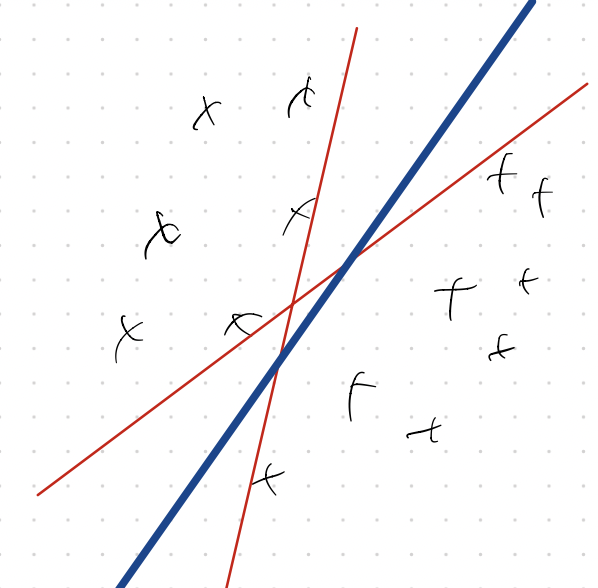
Assume that the data is linearly separable. Then, we can write down the desired classifer as the solution to the following optimization problem (and in classical ML, we call such a model a perceptron.)

or, equivalently,

However, as is the case in the picture above, there could be several linear models that exactly interpolate the labels, which means that the above optimization problem may not have unique solutions. Which solution, then, should we pick?

One way to resolve this issue is by the Large Margin Hypothesis, which asserts that:

Larger margins --> better generalization.

Suppose we associate each linear classifier with the corresponding separating hyperplane (marked in red above). Since we want “most” points in the data space to be correctly classified, a reasonable choice is to find the hyperplane that is furthest away from either class. An easy calculation (shown, for example, here) shows that for any hyperplane parameterized by $w$, the margin equals $\frac{2}{\lVert w \rVert}$. Therefore, maximizing the margin is the same as solving the the optimization problem:

The solution to this problem is called the support vector machine (SVM). This is fine, as long as the data is linearly separable. If not, the constraint set is empty and the optimization problem is ill-posed. A remedy is to relax the (hard) constraints using Lagrange. We get the soft-margin SVM as a solution to the (relaxed) problem:

where $C > 0$ is some weighting parameter, and $l : \R \rightarrow \R$ is some (scalar) loss function that penalizes large negative inputs and leaves inputs bigger than 1 untouched. The $\exp$ loss ($l(z) = e^{-z}$), or the Hinge loss ($l(z) = \max(0,1-z)$) are examples.

Notice that the relaxed problem resembles the standard setup in statistical inference. There is a training loss function $L(w) = \sum_{i=1}^n l(y_i \lang w, x_i \rang)$ and a regularizer $R(w) = \lVert w \rVert^2$, and we seek a model that tries to minimize both. The $\ell_2$-regularizer used above (in deep learning jargon) is sometimes called “weight decay” but others (such as the $\ell_1$-regularizer) are also popular.

An alternative way to arrive at this standard setup is by invoking Occam’s Razor: among the many explanations to the data, we want the one that is of “minimum complexity”. This also motivates a formulation for linear regression which is the same except we use the least-squares loss. Setting $X \in \R^{n \times d}$ as the data matrix, we get:

which is sometimes called Tikhonov regularization. Different choices of $\mu$ lead to different solutions: a large $\mu$ reduces the data fit error, while a small $\mu$ encourages lower-norm solutions.

[There is a long history here which we won’t recount. See here¹ for a nice introduction to the area, and here² which establishes formal generalization bounds in terms of the margin.

However.

In deep learning, anecdotally we seem to be doing just fine even without any regularizers. While regularization may help in some cases, several careful experiments³ show that regularization is neither necessary nor sufficient for good generalization. Why is that the case?

To resolve this, a large body of recent work (which we introduce below) studies what I will call the Algorithmic Bias Hypothesis. This hypothesis asserts that the dynamics of the training procedure (specifically, gradient descent) implicitly introduces a regularization effect. That is, the algorithm itself is biased towards the choice of solution towards minimum complexity solutions, and therefore the explicit imposition of a regularizer is unnecessary.

Remark The results we will prove below hold for both GD as well as SGD, so there is nothing inherently special about the stochasticity of the training procedure. The literature is split on this issue, and I am not aware of compelling theoretical benefits of SGD beyond a per-iteration computational speedup. Indeed, even empirical evidence seems to suggest that stochastic training does not provide any particular benefits from the generalization perspective⁴.

Implicit bias of GD/SGD for linear models

Let’s stick with linear models for a bit longer, since the math will be instructive. We start with the setting of linear regression. We are given a dataset $X = \lbrace (x_i,y_i)_{i=1}^n \subset \R^d \times \R \rbrace$. We assume that the model is over-parameterized, so the number of parameters is greater than the number of examples $(n < d)$. We would like to fit a linear model $u = \langle w, x \rangle$ that exactly interpolates the training data. If we focus on the squared error as the loss function of choice, we seek a (global) minimizer of the loss function:

But note that due to over-parameterization, the data matrix is short and wide, and there are many, many candidate models that achieve zero-loss (indeed, an infinity of them, assuming that the data is in general position.) This is where classical statistics would invoke Occam’s Razor, or margin theory, or such and start introducing regularizers.

Let us blissfully ignore such suggestions, and instead, starting from $w_0 = 0$, run gradient descent on the un-regularized loss $L(w)$. (To be precise, we will run gradient flow, i.e., with infinitesimally small step size – but similar conclusions can be derived for finite but small step sizes, or for stochastic minibatches, with extra algebra.) Therefore, at any time $t$, we have the gradient flow (GF) ordinary differential equation:

We have the following:

Lemma Gradient flow over the squared error loss converges to the minimum $\ell_2$-norm interpolator: \(\begin{aligned} w^* = \arg \min_w \lVert w \rVert^2,~\text{s.t.}~y = Xw. \end{aligned}\) In other words, GF provides an implicit bias towards an $\ell_2$-regularized solution.

Proof This fact is probably folklore, but a proof can be found in Zhang et al.³. We only need one key fact: because we are using the squared error loss, at any time $t$ the gradient looks like:

which is always a vector in the span of the data points. This means that if $w(0) = 0$, then the weights at any time $t$ continues to remain in this span. (Geometrically, the span of the data forms an $n$-dimensional subspace in the $d$-dimensional weight space, so the invariance being preserved here is that the path of gradient descent always lies within this subspace.)

Now, assume that GF converges to a global minimizer, $\bar{w}$. We need to be a bit careful and actually prove that global convergence happens. But we already know that GF/GD minimizes convex loss functions, so let us not repeat the calculations from Chapter 4. Therefore, $\bar{w} = X^T \alpha$ for some set of coefficients $\alpha$. But we also know that since $\bar{w}$ is a global minimizer, $X\bar{w} = y$, which means that

where the inverse exists since the data is in general position. Therefore,

\(\bar{w} = X^T (XX^T)^{-1} y\) which is the Moore-Penrose inverse, or pseudo-inverse, of $X$ applied to $y$. From basic linear algebra we know that the pseudo-inverse gives the minimum-norm solution to the linear system $y = Xw$.

Remark The above proof is algebraic, but there is a simple geometric intuition. Gradient flowlines are orthogonal to the subspace of all possible solutions. Therefore, if we start gradient flow from the origin, then the shortest path to the set of feasible solutions is the straight line segment orthogonal to this subspace, which means that the final answer is the interpolator with minimum $L_2$ norm.

Great! For the squared error loss, the path of gradient descent always leads to the lowest-norm solution, regardless of the training dataset.

Does this intuition carry over to more complex settings? The answer is yes. Let us now describe a similar result (proved here⁵ and here⁶) for the setting of linear classification. Given a linearly separable training dataset, we discover an interpolating classifier using gradient descent over the $\exp$ loss. (This result also holds for the logistic loss.) Somewhat surprisingly, we show that the limit of gradient descent (approximately) produces the min-norm interpolator, which is nothing but the (hard margin) SVM!

The exact theorem statement needs some motivation. For that, let’s first examine the $\exp$ loss, which is somewhat of a strange beast. As defined above, this looks like:

A bit of reflection will suggest that the infimum of $L$ is indeed 0, but ‘zero-loss’ is attained only when the norm of $w$ diverges to infinity. (Exercise: Prove this.) Therefore, we will need to define ‘convergence’ a bit more carefully. The right way to think about it is to look at convergence in direction; for linear classification, the norm of $w$ does not really matter — so we can examine the properties of $\lim w(t)/\lVert w(t) \rVert$ as $t \rightarrow \infty$. We obtain the following:

Theorem Let $w^*$ be the hard-margin SVM solution, or the minimum $\ell_2$-norm interpolator:

Then, gradient flow over the $\exp$ loss converges to:

Moreover,

In other words, GF directionally converges towards the $\ell_2$-max margin solution.

Proof sketch (Complete.)

Remark Convergence happens, but at rate $\frac{1}{\log (t)}$, which is way slower than all the rates we showed in Chapter 4. (Prove this?)

Therefore, we have seen that in linear models, gradient flow induces implicit $\ell_2$-bias for:

• the squared error loss, and
• the $\exp$ loss (as well as the logistic loss⁵.)

What about other choices of loss? Ji et al.⁷ showed a similar directional convergence result for general exponentially tailed loss functions, while clarifying that the limit direction may differ across different losses.

More pertinently, what about other choices of architecture (beyond linear models)? We examine this next.

Implicit bias in multilinear models

The picture becomes much more murky (and, frankly, really fascinating) when we move beyond linear models. As we will show below the architecture plays a fundamental role in the gradient dynamics, which further goes to show that both representation and optimization method play a crucial role in inducing algorithmic bias.

A linear model of the form $u = \lang w, x \rang$ can be viewed as a single neuron with linear activation. Let us persist with linear activations for some more time, but graduate to multiple layers of neurons. One such model is called a two-layer diagonal linear network model:

where the weights $(u_j, v_j)$ are trainable. This model, of course, is merely a re-parameterization of a single neuron and can only express linear functions. However, the weights interact multiplicatively, and therefore the output is a nonlinear function of the weights. This re-parameterization makes a world of difference in the context of gradient dynamics, and leads to a very different form of algorithmic bias, as we will show below.

Diagonal linear models

For simplicity, let’s just assume that the weights are tied across layers, i.e., $u_i = v_i$ for $i \in [d]$. I don’t believe that this assumption is important; similar conclusions should hold even if no weight tying occurs.

Then, the prediction for any data point $x \in \R^d$ becomes

or if we stack up the training data then

where $\circ$ denotes the element-wise (Hadamard) product. This is called a “two-layer diagonal linear network”, and the extension to $L$-layers is analogous. Notice that by using this re-parameterization, we have not done very much in terms of expressiveness.

(Actually, the last statement is not very precise; square reparameterization only expresses linear models $y = Xw$, but with the added restriction that $w \geq 0$. But this can be fixed easily as follows: introduce 2 sets of variables $u$ and $v$, and write $y = X(u\circ u - v\circ v)$.)

Let’s stick with the squared error loss:

and suppose we perform gradient flow over this loss. Since $L$ is a fourth-order polynomial (quartic) function of $u$, the ODE governing the gradient at any time instant is a bit more complicated:

Notice now that the gradient in fact is now a cubic function of $u$. Suppose that we initialize $u = \alpha \mathbf{1}$, where $\mathbf{1}$ is the all-ones vector and $\alpha > 0$ is a scalar. (This is fine since in the end we will only be interested in models with positive coefficients.)

Somewhat curiously, we can prove that if $\alpha$ is small enough then the algorithmic bias corresponding to gradient flow corresponds to $\ell_1$-regularization (i.e., we recover the familiar basis pursuit or Lasso formulation. Formally, we get the following:

Theorem Let $w^*$ be the (non-negative) interpolator with minimum $\ell_1$-norm:

Suppose that gradient flow for diagonal linear networks converges to an estimate $\bar{u}$. Then $\bar{w} = \bar{u} \circ \bar{u}$ converges to $w^*$ as $\alpha \rightarrow 0$.

Proof sketch This proof is by Woodworth et al.⁸ Let us give high level intuition first. It will be helpful to understand two types of dynamics: one in the original (canonical) linear parameterization in terms of $w$, and the other in the square re-parameterization (in terms of $u$). By definition, we have $w_j = u_j^2$, and therefore

By plugging in the definition of gradient flow, we get:

This resembles gradient flow over the standard $\ell_2$-loss, except that each coordinate is multiplied with $w_i(t)$. Intuitively, this induces a “rich-get-richer” phenomenon: a bigger coefficient in $w(t)$ is assigned a larger gradient update (relative to the other coefficients) and therefore “moves” towards its final destination faster.

Gissin et al.⁹ call this incremental learning: large coefficients are learned (approximately) in decreasing order of their magnitude. (See their paper/website for some terrific visualizations of the dynamics.)

To rigorously argue that the bias indeed is the $\ell_1$-regularizer, let $e(t) = y - X w(t)$ denote the prediction error at any time instant. Then, as shown above, we have the ODE:

Solving this equation coordinate-wise, we get the closed form solution:

Plugging in the initialization $u(0) = \alpha \mathbf{1}$ and $w(t) = u(t) \circ u(t)$, we get:

Therefore, assuming the dynamics converges (technically we need to prove this, but let’s sweep that under the rug for now), we get that the limit of gradient flow gives:

where $f$ is a coordinate-wise function such that $f(z):= \alpha^2 \exp(z)$ and $\lambda := 4 \int_0^\infty e(s) ds$. Since $\alpha > 0$, $f$ is bijective and therefore

Now, assume that the algorithmic bias of GF can be expressed by some unique regularizer $Q(w)$. (Again, we are making a major assumption here that the bias is expressible in the form of a well-defined function of $w$, but let’s do more rug+sweeping here.) We will show that $Q(w)$ approximately equals the $\ell_1$-norm of $w$. We get:

KKT optimality tells us that the optimum ($\bar{w}$) should satisfy:

for some vector $\lambda$. Therefore, we can reverse-engineer $Q$ by solving the differential equation:

This (again) has the closed form solution:

Therefore, as $\alpha \rightarrow 0$, the first term starts to (significantly) dominate the second, and we can therefore write:

due to the fact that $w$ is non-negative by definition.

Remark The above proof shows (again) that the algorithmic bias of gradient descent highly depends on the initialization; the fact that $\alpha \rightarrow 0$ was crucial in establishing $\ell_1$-bias. On the other hand, a different initialization with $\alpha \rightarrow \infty$ leads to a completely different bias: GF automatically provides $\ell_2$-regularization.⁸ Woodworth et al. categorize these two distinct behaviors of gradient descent as respectively operating in the “rich” and “kernel” regimes.

Remark The fact that $u(0)$ was initialized with a constant vector (with magnitude $\alpha$) is unimportant; one can impose different forms of bias with varying choices (or “shapes”) of the initialization¹⁰.

Remark At its core, the net effect of square reparameterization is to alter the optimization geometry of gradient descent. This can be connected to classical optimization theory in general Banach spaces, and indeed the dynamics of diagonal linear networks can be viewed as a form of mirror descent (MD). See here¹¹ and here¹² for a more thorough treatment.

Remark All of the above assume that the limit of gradient flow admits an exact interpolation. In the presence of noise in the labels the situation is a bit more subtle, and a more careful analysis of the ODEs is necessary; in some cases, for consistent generalization, early stopping may be necessary. See our paper for details¹³.

Remark (Two-layer dense nets and nuclear norm regularization) (complete).

Implicit bias of gradient descent in nonlinear networks

As we saw above, changing the architecture fundamentally changes the gradient dynamics (and therefore the implicit regularization induced during training.) But our discussion above focused on networks with linear activations. How does the picture change with more standard networks (such as those with ReLU activations?)

Not surprisingly, life becomes harder when dealing with nonlinearities. Yet, the tools above pave a way to understand algorithmic bias for such networks. Let’s start simple and work our way up.

Single neurons

Consider a network consisting of a single neuron with nonlinear activation $\psi : \R \rightarrow \R$. The model becomes:

and we will use the squared error loss to train it:

where $X$ is the data matrix. We train the above (single-neuron) network using gradient flow. The following proof is by Vardi and Shamir¹⁴.

Theorem Suppose that $\psi : \R \rightarrow \R$ is a monotonic function. If gradient flow over $L(w)$ converges to zero loss, then the limit $\bar{w}$ automatically satisfies:

In other words, GF provides an implicit bias towards an $\ell_2$-regularized solution.

Proof Reduce to linear case using monotonicity. (complete)

Activation functions such as leaky-ReLU, sigmoid etc do satisfy monotonicity. (For sigmoid, convergence to zero loss is a bit tricky because of non-convexity.) What about the regular ReLU? This is more difficult, and there does not appear to be a clean “norm”-based regularizer.

Multiple layers

Two-layer nets. complete.