Chapter 5 - Optimizing wide networks

In the previous chaper, we proved that (S)GD converges locally for training neural networks with smooth activations. (The case for ReLU networks is harder but still doable with additional algebraic heavy lifting.)

However, in practice, somewhat puzzlingly we encounter very deep networks that are regularly optimized to zero training loss, i.e., they exactly learn to interpolate the given training data and labels. Since loss functions are typically non-negative, this means that (S)GD have achieved convergence to the global optimum.

In this chapter, we ask the question:

When and why does (S)GD give zero train loss?

An answer to this question in full generality is not yet available. However, we will prove a somewhat surprising fact: for very wide networks that are randomly initialized, this is indeed the case. The road to proving this will give us several surprising insights, and connections to classical ML (such as kernel methods) will become clear along the way.

Local versus global minima

Let us bring up this picture from Xu et al.¹ again:

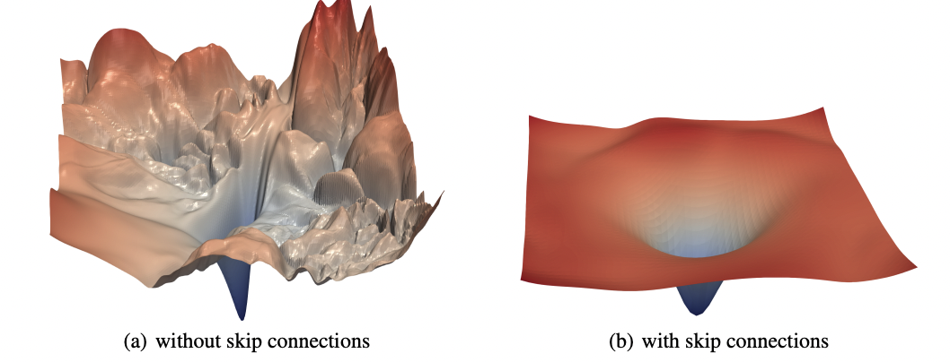
The picture on the left shows the loss landscape of a feedforward convolutional network. The picture on the right shows the loss landscape of the same network with residual skip connections.

Why would (S)GD navigate its way to the global minimum of this jagged-y, corrugated loss landscape? There could be one of many explanations.

• Explanation 1: We got lucky and initialized very well (close enough to the global optimum for GD to work). But if there is only one global minimum then “getting lucky” is an event that happens with exponentially small probability. So there has to be another reason.

• Explanation 2: The skips (clearly) matter, so maybe most real-world networks in fact look like the ones on the right. There is a grain of truth here: in modern (very) deep networks, there exist all kinds of bells and whistles to “make things work”. Residual (skip) connections are common. So are other tweaks such as batch normalization, dropout, learning rate scheduling, etc etc. All² of these³ tweaks⁴ significantly influence the nature of the optimization problem.

• Explanation 3: Since modern deep networks are so heavily over-parameterized, there may be tons of minima that exactly interpolate the data. In fact, with high probability, a random initialization lies “close” to a interpolating set of weights. Therefore, gradient descent starting from this location successfully trains to zero loss.

We will pursue Explanation 3, and derive (mathematically) fairly precise justifications of the above claims. As we will argue in the next chapter, this is by no means the full picture. But the exercise is still going to be very useful.

The Neural Tangent Kernel

Our goal will be to understand what level of over-parameterization enables gradient descent to train neural network models to zero loss. So if the network contains $p$ parameters, we would like to derive scaling laws of $p$ in terms of $n$ and $d$. Since the number of parameters is greater than the number of samples, proving generalization bounds will be challenging. But let’s set aside such troubling thoughts for now.

When we think of modern neural networks and their size, we typically associate “growing” the size of networks in terms of their depth. However, our techniques below will instead focus on the width of the network (mirroring our theoretical treatment of network representation capacity). Many results below apply to deep networks, but the key controlling factor is the width (note: actually, not even the width but other strange properties; more later.) The impact of depth will continue to remain elusive.

Here’s a high level intuition of the path forward:

1. We know that if the loss landscape is convex, then the dynamics of training algorithms such as GD or SGD ensures that we always converge to a global optimum.

2. We know that linear/kernel models exhibit convex loss landscapes.

3. We will prove that for wide enough networks, the loss landscape looks like that of a kernel model.

So in essence, establishing the last statement triggers the chain of implications:

and we are done.

Some history. The above idea is called the Neural Tangent Kernel, or the NTK, approach. The term itself first appeared in a landmark paper by Jacot et al.⁵, which first established the global convergence of NN training in the infinite-width limit. Roughly around the same time, several papers emerged that also provided global convergence guarantees in certain specialized families of neural network models. See here⁶, here⁷, and here⁸. All of them involved roughly the same chain of implications as described above, so now can be dubbed as “NTK-style” papers.

Gradient dynamics for linear models

As a warmup, let’s first examine how GD over the squared-error loss learns the parameters of linear models. Most of this should be classical. For a given training dataset $(x_i, y_i)$, define the linear model using weights $w$, so that the predicted labels enjoy the form:

where $X$ is a matrix with the data points stacked row-wise. This leads to the familiar loss:

We optimize this loss via GD:

where the gradient of the loss looks like:

and so far everything is good. Now, imagine that we execute gradient descent with infinitesimally small step size $\eta \rightarrow 0$, which means that we can view the evolution of the weights as the output of the following ordinary differential equation (ODE):

This is sometimes called Gradient Flow (GF), and standard GD is rightfully viewed as a finite-time discretization of this ODE. Moreover, due to linearity of the model, the evolution of the output labels $u$ follows the ODE:

Several remarks are pertinent at this point:

• Linear ODEs of this nature can be solved in closed form. If $r = y-u$ is the “residual” then the equation becomes:

  \[\frac{dr}{dt} = - H r\]

  whose solution, informally, is the (matrix) exponential:

  \[r(t) = \exp(-Ht) r(0)\]

  which immediately gives that if $H$ is full-rank with $\lambda_{\text{min}} (H) >0$, then GD is extremely well-behaved; it provably converges at an exponential rate towards a set of weights with zero loss.

• Following up from the first point: the matrix $H = X X^T$, which principally governs the dynamics of GD, is constant with respect to time, and is entirely determined by the geometry of the data. Configurations of data points which push $\lambda_{\text{min}} (H)$ as high as possible enable GD to converge quicker, and vice versa.

• The data points themselves don’t matter very much; all that matters is the set of their pairwise dot products:

  \[H_{ij} = \langle x_i, x_j \rangle .\]

  This immediately gives rise to an alternate way to introduce the well-known kernel trick: simply replace $H$ by any other easy-to-compute kernel function:

  \[K_{ij} = \langle \phi(x_i), \phi(x_j) \rangle\]

  where $\phi$ is some feature map. We now suddenly have acquired the superpower of being able to model non-linear features of the data. This derivation also shows that training kernel models is no more challenging than training linear models (provided $K$ is easy to write down.)

Gradient dynamics for general models

Let us now derive the gradient dynamics for a general deep network $f(w)$. We mirror the above steps. For a given input $x_i$, the predicted label obeys the form:

where the subscript of $f$ here makes the dependence on the input features explicit. The squared-error loss becomes:

and its gradient with respect to any one weight becomes:

Therefore, the dynamics of any one output label – which, in general, depends on all the weights – can be calculated by summing over the partial derivatives over all the weights:

where in the last step we switched the orders of summation, and defined:

We have used angular brackets to denote dot products. In the case of an infinite number of parameters, the same relation holds. But we have to replace summations by expectations over a measure (and perform additional algebra book-keeping, so let’s just take it as true).

Once again, we make several remarks:

• Observe that the dynamics is very similar in appearance to that of a linear model! in vector form, we get the evolution of all $n$ labels as

  \[\frac{du}{dt} = H_t (y - u)\]

  where $H_t$ is an $n \times n$ matrix governing the dynamics.

• But! There is a crucial twist! The governing matrix $H_t$ is no longer constant: it depends on the current set of weights $w$, and therefore is a function of time — hence the really pesky subscript $t$. This also means that the ODE is no longer linear; $H_t$ interacts with $u(t)$, and therefore the picture is far more complex.

• One can check that $H_t$ is symmetric and positive semi-definite; therefore, we can view the above equation as the dynamics induced by a (time-varying) kernel mapping. Moreover, the corresponding feature map is nothing but:

  \[\phi : x \mapsto \frac{\partial f_{x}(w)}{\partial w }\]

  which can be viewed as the “tangent model” of $f$ at $w$. This is a long-winded explanation of the origin of the name “NTK” for the above analysis.

Wide networks exhibit linear model dynamics

The above calculations give us a mechanism to understand how (and under what conditions) gradient dynamics of general networks resemble those of linear models. Basically, our strategy will be as follows:

1. We will randomly initialize weights at $t=0$.

2. At $t=0$, we will prove that the corresponding NTK matrix, $H_0$, is full-rank and that its eigenvalues are bounded away from zero.

3. For large widths, we will show that $H_t \approx H_0$, i.e., the NTK matrix stays approximately constant. In particular, the dynamics always remains full rank.

Combining $1+2+3$ gives the overall proof. This proof appeared in Du et al.⁶ and the below derivations are adapted from this fantastic book ⁹.

Concretely, we consider two-layer networks with $m$ hidden neurons with twice-differentiable activations $\psi$ with bounded first and second derivatives. This again means that ReLU doesn’t count, but other analogous proofs can be derived for ReLUs; see⁶.

For ease of derivation, let us assume that the second layer weights are fixed and equal to $\pm 1$ chosen equally at random, and that we only train the first layer. This assumption may appear strange, but (a) all proofs will go through if we train both layers, and (b) the first layer weights are really the harder ones in terms of theoretical analysis. (Exercise: Show that if we flip things around and train only the second layer, then really we are fitting a linear model to the data.)

Therefore, the model assumes the form:

where $a_r = \pm 1$ and the scaling $\frac{1}{\sqrt{m}}$ is chosen to make the algebra below nice. (Somewhat curiously, this exact scaling turns out to be crucial, and we will revisit this point later.)

We initialize all weights $w_1(0), w_2(0), \ldots, w_r(0)$ according to a standard normal distribution. In neural network Since we are only using 2-layer feedforward networks, the gradient at time $t=0$ becomes:

with respect to the weights of the $r^{th}$ neuron. As per our above derivation, at time $t=0$, we get that the NTK has entries:

There is quite a bit to parse here. The main point here is to note that each entry of $H(0)$ is the average of $m$ random variables whose expectation equals:

In other words, if we had infinitely many neurons in the hidden layer then the NTK at time $t=0$ would equal its expected value, given by the matrix $H^$. (Exercise: It is not hard to check that for $m = \Omega(n)$ and for data in general position, $H^$ is full rank; prove this.)

Our first theoretical result will be a bound on the width of the network that ensures that $H(0)$ and $H^*$ are close.

Theorem Fix $\varepsilon >0$. Then, with high probability we have

provided the hidden layer has at least

neurons.

Our second theoretical result will be a width bound that ensures that $H(t)$ remains close to $H(0)$ throughout training.

Theorem Suppose that $y_i = \pm 1$ and $u_i(\tau)$ remains bounded throughout training, i.e., for $0 \leq \tau < t$. Fix $\varepsilon >0$. Then, with high probability we have

provided the hidden layer has at least

neurons.

Before providing proofs of the above statements, let us make several more remarks.

• The above results show that the width requirement scales polynomially with the number of samples. (In fact, it is a rather high degree polynomial.) Subsequent works have tightened this dependence; these¹⁰ papers¹¹ were able to achieve a quadratic scaling of $m = \tilde{O}(n^2)$ hidden neurons for GD to provably succeed. As far as I know, the current best bound is sub-quadratic ($O(n^{\frac{3}{2}})$), using similar arguments as above; see here¹².

• The above derivation is silent on the dimension and the geometry of the input data. If we assume additional structure on the data, we can improve the dependence to $O(nd)$; see our paper¹³. However, the big-oh here hides several data-dependent constants that could become polynomially large themselves.

• For $L$-layer networks, the best available bounds are rather weak; widths need to scale as $m = \text{poly}(n, L)$. See here⁷ and here¹⁴.

Lazy training

** (Complete) **

Proofs

** (COMPLETE) **.