Chapter 1 - Memorization

Let us begin by trying to rigorously answer a very simple question:

How many neurons suffice?

Upon reflection it should clear that this question isn’t well-posed. Suffice for what? For good performance? On what task? Do we even know if this answer is well-defined – perhaps it depends on some hard-to-estimate quantity related to the learning problem? Even if we were able to get a handle on this quantity, does it matter how the neurons are connected – should the network be wide/shallow, or narrow/deep?

Let us begin simple. Suppose all we have is a bunch of training data points: \[ X = \lbrace (x_i, y_i)\rbrace_{i=1}^n \subset \mathbb{R}^d \times \mathbb{R} \] and our goal will be to discover a network that exactly memorizes $X$. That is, we will learn a function $f$ that, when evaluated on every data point $x_i$ in the training data, returns $y_i$. Equivalently, if we define empirical risk via the squared error loss:

then $f$ achieves zero empirical risk. Our intuition says (and we will prove more versions of this later) is that a very large (very wide, or very deep, or both) network is likely enough to fit basically anything we like. So really, we want reasonable upper bounds on the number of neurons needed for exact memorization.

But why should we care about memorization anyway? After all, machine learning folks are taught to be wary of overfitting to the training set. In introductory ML courses we spend several hours (and homework sets) covering the bias-variance tradeoff, the importance of adding a regularizer to decrease variance (at the expense of incurring extra “bias”), etc etc.

Unfortunately, deep learning practice throws this classical way of ML thinking out of the window. We seldom use explicit regularizers, instead relying on standard losses. We typically train deep neural networks to achieve 100\% (train) accuracy. Later, we will try to understand why networks trained to perfectly interpolate the training data still generalize well, but for now let’s focus on just achieving a representation that enables perfect memorization.

Basics

First, a basic definition of a “neural network”.

For our purposes, neural network is composed of several primitive “units”, each of which we will call a neuron. Given an input vector $x \in \mathbb{R}^d$, a neuron transforms the input according to the following functional form:

Here, $w_j$ are the weights, $b$ is a scalar called the bias, and $\psi$ is a nonlinear scalar transformation called the activation function; a typical activation function is the “ReLU function” $\psi(z) = \max(0,z)$ but we will also consider others.

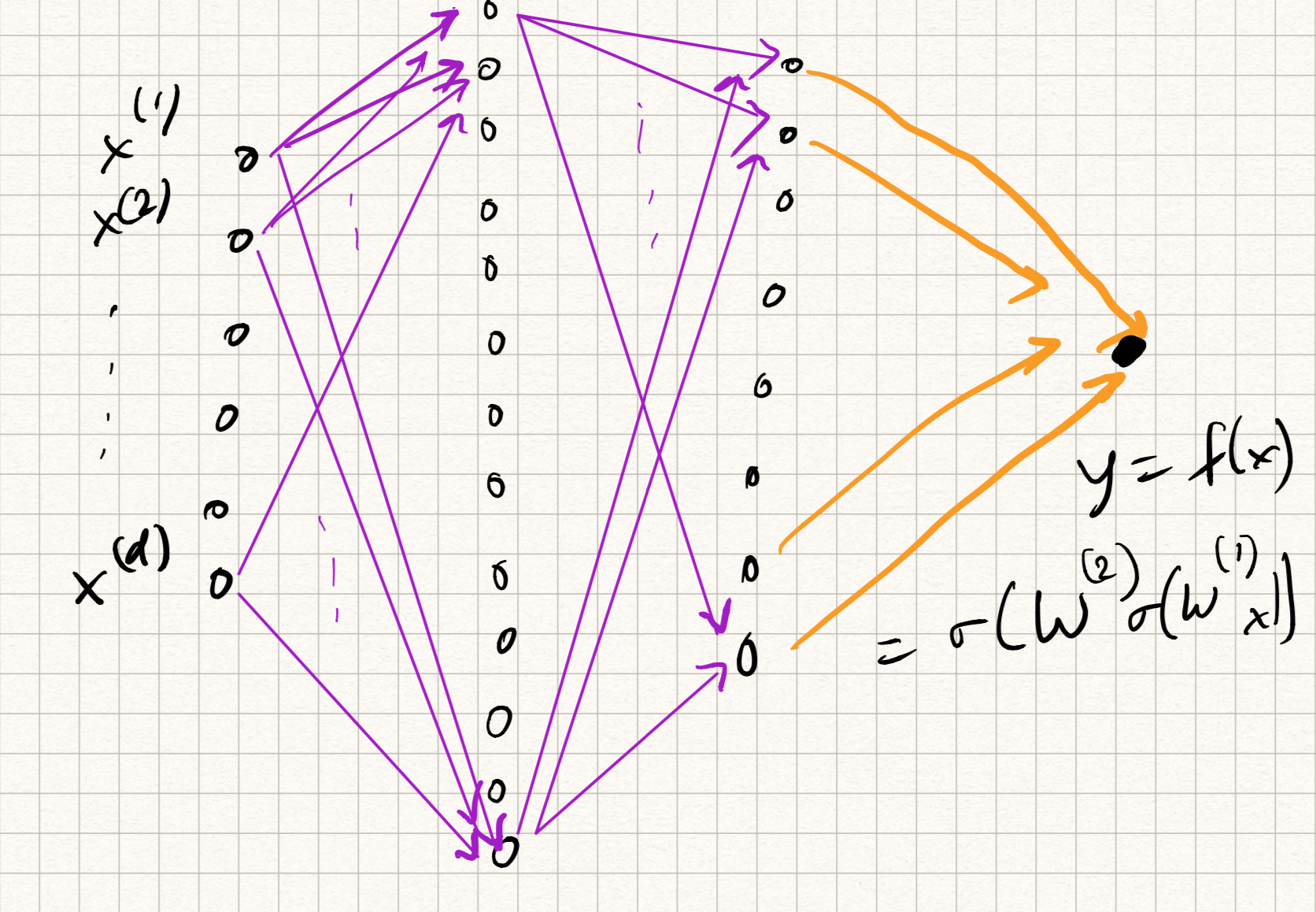
A neural network is a feedforward composition of several neurons, typically arranged in the form of layers. So if we imagine several neurons participating at the $l^{\text{th}}$ layer, we can stack up their weights (row-wise) in the form of a weight matrix $W^{(l)}$. The output of neurons forming each layer forms the corresponding input to all of the neurons in the next layer. So a neural network with two layers of neurons would have

Analogously, one can extend this definition to $L$ layers for any $L \geq 1$. The nomenclature is a bit funny sometimes. The above example is either called a “3-layer network” or “2-hidden-layer network”, depending on who you ask. The output $y$ is considered as its own layer and not considered as “hidden” (also notice that it doesn’t have any activation in this case; that’s typical.)

Memorization capacity: Standard results

A lot of interesting quirks arise even in the simplest cases.

Let us focus our attention on the ability of two-layer networks (or one-hidden-layer networks) to memorize $n$ data points. We will restrict discussion to ReLU activations but the arguments below are generally applicable. If there are $m$ hidden neurons and if $\psi$ is the ReLU then our hypothesis class $\f_m$ comprises all functions $f$ such that for suitable weight parameters $(\alpha_i, w_i)$ and bias parameters $b_i$, we have:

\[ f(x) = \sum_{i=1}^m \alpha_i \psi(\langle w_i, x \rangle + b_i) . \]

Intuitively, $m < \infty$ is a trivial upper bound on any dataset (we will be more rigorous about this when we prove universal approximation results). If we have infinitely many parameters then memorization should be trivial. Let us get a better upper bound for $m$. Our first result shows that $m = n$ should suffice.

Theorem Let $f$ be a two-layer ReLU network with $m = n$ hidden neurons. For any arbitrary dataset $X = \lbrace (x_i, y_i)_{i=1}^n\rbrace \subset \mathbb{R}^d \times \mathbb{R}$ where $x_i$ are in general position, the weights and biases of $f$ can be chosen such that $f$ exactly interpolates $X$.

Proof This result is non-constructive and seems to be folklore, dating back to at least Baum¹. For modern versions of this proof, see Bach² or Bubeck et al.³.

Define the space of arbitrary width two-layer networks: \[\f = \bigcup_{m \geq 0} \f_m . \] The high level idea is that $\f$ forms a vector space. This is easy to see, since it is closed under additions and scalar multiplications. Formally, fix $x$ and consider the element $\psi_{w,b}: x \mapsto \psi(\langle w, x \rangle + b)$. Then, $\text{span}(\psi_{w,b})$ forms a vector space. Now, consider the linear pointwise evaluation operator $\Psi : V \rightarrow \mathbb{R}^n$: \[\Psi(f) = (f(x_1), f(x_2), \ldots, f(x_n)) .\] We know from classical universal approximation (Chapter 2) that every vector in $\mathbb{R}^n$ can be written as some (possibly infinite) combination of neurons. Therefore, $\text{Range}(\Psi) = \mathbb{R}^n$, or $\text{dim(Range}(\Psi)) = n$. Therefore, there exists some basis of size $n$ with the same span! Call this basis $\lbrace \psi_1, \ldots,\psi_n\rbrace$. This basis can be used to express any set of labels by choosing appropriate coefficients in a standard basis representation $y = \sum_{i=1}^n \alpha_i \psi_i$. The result follows.

In fact, the above result holds for any activation function $\psi$ that is not a polynomial⁴; we will revisit this curious property later.

Really, we didn’t do much here. Since the “information content” in $n$ labels has dimension $n$, we can extract any arbitrary basis (written in the form of neurons) and write down the expansion of the labels in terms of this basis. Since this approach may be a bit abstract, let’s give an alternate constructive proof.

Proof (Alternate.) This proof can be attributed to Zhang et al⁵. Suppose $m = n.$ Since all $x_i$’s are distinct and in general position, we can pick a $w$ such that if define $z_i := \langle w, x_i \rangle$ then without loss of generality (or by re-indexing the data points): \[ z_1 < z_2 < \ldots z_n . \] One way to pick $w$ is by random projection: pick $w$ from a standard $d$-variate Gaussian distribution; then the above holds with high probability. If the above relation between $z_i$ holds, we can find some sequence of $b_i$ such that: \[ b_1 < z_1 < b_2 < z_2 < \ldots < b_n < z_n . \] Now, let’s define an $n \times n$ matrix $A$ such that \[ A_{ij} := \text{ReLU}(z_i - b_j) = \max(z_i - b_j, 0) . \] Since by definition, each $z_i$ is only bigger than all $b_j$ for $1 \leq j \leq i$, we have that $A$ is a lower triangular matrix with positive entries on the diagonal, and therefore full rank. Moreover, for any $\alpha \in \mathbb{R}^n$, the product $A \alpha$ is the superposition of exactly $n$ ReLU neurons (the weights are the same for all of them, but the biases are distinct). Set $\alpha = A^{-1} y$ and we are done.

Remark The above proofs used biases, but if we restrict our attention to bias-free networks, that’s fine too, we just need to use different weights for the $n$ hidden neurons. Such a network is called a random feature model; see here and here.

Memorization capacity: Improved results

The above result shows that $m = n$ neurons are sufficient to memorize pretty much any dataset. Can we get away with fewer neurons? Notice that really the network has to “remember” only the $n$ labels; but since there are $n$ neurons, each with $d$ input edges, the number of parameters is $nd$. (Note: not technically correct; the second proof only uses $n$ distinct weights and $n$ biases.) It turns out that we can indeed do better.

Theorem For any dataset of $n$ points in general position, $m = 4 \lceil \frac{n}{d} \rceil$ neurons suffice to memorize it.

Proof For ReLU activations, this proof is in Bubeck et al³, although Baum¹ proved a similar result for threshold activations and binary labels.

Notice that $d = \Omega(1)$ is actually beneficial here; higher input dimension implies easier memorization. In some ways this is a blessing of dimensionality phenomenon.

We will prove Baum’s result first. Suppose we have threshold activations (i.e., $\psi(z) = \mathbb{I}(z \geq 0)$) and binary labels $y_i \in \pm {1}$. We iteratively build a network as follows. Without loss of generality, we can assume that there are at least $d$ points with label equal to $y_i = 1$; index them as $x_1, x_2, \ldots, x_d$. Since the points are in general position, we can find an affine subspace that exactly interpolates these points:

and record $(w_1, b_1)$. (Importantly, again since the points are in general position no other points lie in this subspace.)

Now, form a very thin indicator slab using for this affine subspace using exactly two neurons:

for some small enough $\varepsilon > 0$. This function is equal to 1 for exactly the points in the subspace, and zero for all other points. For this group of $d$ points we can assign the output weight $\alpha_1 = 1$. Iterate this argument $\lceil \frac{n}{d} \rceil$ times and we are done! Therefore, $2 \lceil \frac{n}{d} \rceil$ threshold neurons suffice if the labels are binary.

The exact same argument can be extended to ReLU activations and arbitrary (scalar) labels. Again, we iteratively build the network. We pick an arbitrary set of $d$ points, through which we can interpolate an affine subspace:

We now show that we can memorize these $d$ data points using 4 ReLU neurons. The trick is to look at the “directional derivative” of the ReLU:

As $\delta \rightarrow 0$, the right hand side approaches the quantity:

But: the first part is the “derivative” of the ReLU, which is exactly the threshold function! Using the thin-slab-indicator trick in the proof above, the difference of two such functions (with slightly different $b$) forms an indicator on a thin slab around these $d$ points:

Since we are using differences-of-differences, we need 4 ReLUs to realize $f$. It now remains to pick $v$. But this is easy: since the data are in general position, just solve for $v$ such that

Repeat this fitting procedure $\lceil \frac{n}{d} \rceil$ times and we are done.

Remark The above construction is somewhat wacky/combinatorial. The weights of each neuron was picked myopically (we never revisited data points) and locally (each neuron only depended on a small subset of data points).

Remark The above construction says very little about how large networks need to be in order for “typical” learning algorithms (such as SGD) to succeed. We will revisit this in the Optimization chapters. For a recent result exploring the properties of “typical” gradient-based learning methods in the $O(n/d)$ regime, see here⁶.

Remark All the above results used a standard dense feedforward architecture. Analogous memorization results have been shown for other architectures commonly used in practice today: convnets⁷, ResNets⁸, transformers⁹, etc.

Lower bounds

The above results show that we can memorize $n$ (scalar) labels with no more than $O(n/d)$ ReLU neurons – each with $d$ incoming edges, which means that the number of learnable weights in this network is $O(n)$. Is this upper bound tight, or is there hope for doing any better?

The answer seems to be no, and intuitively it makes sense from a parameter counting perspective. Sontag¹⁰ proved an early result along these lines, showing that if some function $f$ that is described with $o(n)$ parameters is analytic (meaning that it is smooth and has convergent power series) and definable (meaning that it can be expressed by some arbitrary composition of rational operations and exponents), then there exists at least one dataset of $n$ points that the network cannot memorize. This result also holds for functions that are piecewise analytic and definable, meaning that neural networks (of arbitrary depth! not just two layers!) are applicable to this theorem.

(Note: this observation is not technically correct; we can get better by “bit stuffing”. If we assume slightly more restrictive properties on the data and allow the network weights to be unbounded, then this bound can be improved to $O(\sqrt{n})$ parameters. We will revisit this later.)

So it may seem interesting that we were able to get best-possible memorization capacity using simple 2-layer networks. So does additional depth buy us anything at all? The answer for this is yes: we can decrease the number of hidden neurons in the network significantly when we move from 1- to 2-hidden-layer networks. We will revisit this in Chapter 3.

Robust interpolation

(Complete)