Chapter 2 - Universal approximators

Previously, we visited several results that showed how (shallow) neural networks can effectively memorize training data. However, memorization of a finite dataset may not the end goal¹. In the ideal case, we would like to our network to simulate a (possibly complicated) prediction function that works well on most input data points. So a more pertinent question might be:

Can neural networks simulate arbitrary functions?

In this note we will study the representation power of (shallow) neural networks through the lens of their ability to approximate (continuous) functions. This line of work has a long and rich history. The field of function approximation, independent of the context of neural networks, is a vast body of work which we can only barely touch upon. See here² for a recent (and fantastic) survey.

As before, intuition tells us that an infinite number of neurons should be good enough to approximate pretty much anything. Therefore, our guiding principle will be to achieve as succinct a neural representation as possible. Moreover, if there is an efficient computational routine that gives this representation, that would be the icing on the cake.

Warmup: Function approximation

Let’s again start simple. This time, we don’t have any training data to work with; let’s just assume we seek some (purported) prediction function $g(x)$. To approximate $g$, we have a candidate hypothesis class $\f_m$ of shallow (two-layer) neural networks of the form:

\[ f(x) = \sum_{i=1}^m \alpha_i \psi(\langle w_i, x \rangle + b_i) . \]

Our goal is to get reasonable bounds on how large $m$ needs to be in terms of various parameters of $g$. We have to be clear about what “approximate” means here. It is typical to measure approximation in terms of $p$-norms between measurable functions; for example, in the case of $L_2$-norms we will try to control

where $\mu$ is some measure defined over $\text{dom}(g)$. Likewise for the $L_\infty$- (or the sup-)norm, and so on.

Univariate functions

We begin with the special case of $d=1$ (i.e., the prediction function $g$ is univariate). Let us first define a useful property to characterize univariate functions.

Definition (Univariate Lipschitz.) A function $g : \R \rightarrow \R$ is $L$-Lipschitz if for all $u,v \in \R$, we have that $|f(u) - f(v) | \leq L |u - v|$.

Why is this an interesting property? Any smooth function with bounded derivative is Lipschitz; in fact, certain non-smooth functions (such as the ReLU) are also Lipschitz. Lipschitz-ness does not quite capture everything we care about (e.g. discontinuous functions are not Lipschitz, which can be somewhat problematic if there are “jumps” in the label space). But it serves as a large enough class of functions to prove interesting results.

An additional benefit of Lipschitzness is due to approximability. If our target function $f$ is $L$-Lipschitz with reasonable $L$, then we can show that it can be well-approximated by a two-layer network with threshold activations: $\psi(z) = \mathbb{I}(z \geq 0)$. We prove:

Theorem Let $g : [0,1] \rightarrow \R$ be $L$-Lipschitz. Then, it can be $\varepsilon$-approximated in the sup-norm by a two-layer network with $O(\frac{L}{\varepsilon})$ hidden threshold neurons.

Proof. A more careful derivation of this fact (and the next one below) can be found in Telgarsky³. The proof follows from the same picture we might have seen while first learning about integrals and Riemann sums. The high level idea is to tile the interval $[0,1]$ using “buildings” of appropriate height. Since the derivatives are bounded (due to Lipschitzness), the top of each “building” cannot be too far away from the corresponding function value. Here is a picture:

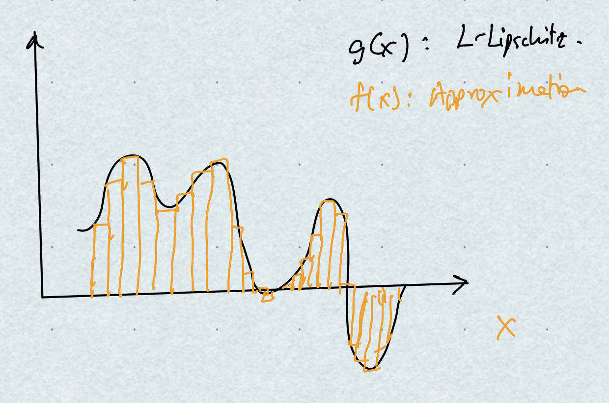
More formally: partition $[0,1]$ into equal intervals of size $\varepsilon/L$. Let the $i$-th interval be $[u_i,u_{i+1})$. Define a sequence of functions $f_i(x)$ where each $f_i$ is zero everywhere, except within the $i$-th interval where it attains the value $g(u_i)$. Then $f_i$ can be written down as the difference of two threshold functions:

Our network will be the sum of all the $f_i$’s (and there are $L/\varepsilon$ of them). Moreover, for any $x \in [0,1]$, if $u_i$ is the left end of the interval corresponding to $x$, then we have:

Taking the supremum over all $x \in [0,1]$ completes the proof.

Remark So we can approximate $L$-Lipschitz functions with $O(L/\varepsilon)$ threshold neurons. Would the answer change if we used ReLU activations? (Hint: no, up to constants; prove this.)

Multivariate functions

Of course, in deep learning we rarely care about univariate functions (i.e., where the input is 1-dimensional). We can ask a similar question in the more general case. Suppose we have $L$-Lipschitz functions over $d$ input variables and we want to approximate it using shallow neural networks. How many neurons do we need?

We answer this question using two approaches. First, we give a construction using standard real analysis that uses two hidden layers of neurons. Then, with some more mathematical powerful machinery we will get better (and much more general) results with only one hidden layer (i.e., using the hypothesis class $\f$).

First, we have to define Lipschitzness for $d$-variate functions.

Definition (Multivariate Lipschitz.) A function $g : \R^d \rightarrow \R$ is $L$-Lipschitz if for all $u,v \in \R^d$, we have that $|f(u) - f(v) | \leq L \lVert u - v \rVert_\infty$.

Theorem Let $g : [0,1]^d \rightarrow \R$ be $L$-Lipschitz. Then, $g$ can be $\varepsilon$-approximated in the $L_1$-norm by a three-layer network $f$ with $O(\frac{L}{\varepsilon^d})$ hidden threshold neurons.

Proof sketch. The proof follows the above construction for univariate functions. We will tile $[0,1]^d$ with equally spaced multidimensional rectangles; there are $O(\frac{1}{\varepsilon^d})$ of them. The value of the function $f$ within each rectangle will be held constant (and due to the definition of Lipschitzness, the error with respect to $g$ cannot be too large). If we can figure out how to approximate $g$ within each rectangle, then we are done.

The key idea is to figure out how to realize “indicator functions” for every rectangle. We have seen that in the univariate case, indicators can be implemented using the difference of two threshold neurons. In the $d$-variate case, an indicator over a rectangle is the Cartesian product over the $d$ axis. however, Boolean/Cartesian products can be implemented by a layer of threshold activations on top of these differences.

Formally, consider any arbitrary piece with $[u_j,v_j), j=1,2,\ldots,d$ as sides. The domain can be written as the Cartesian product:

Therefore, we can realize an indicator function over this domain as follows. Localize within each coordinate by the “difference-of-threshold neurons”:

and implement the entire rectangle is implemented via a “Boolean AND” over all the coordinates:

where $x_j$ is the $j$-th coordinate of $x$. There is one such $h$ for every rectangle, and the output edge from this neuron is assigned a constant value approximating $g$ within that rectangle. This completes the proof.

Remark Would the answer change if we used ReLU activations? (Hint: no, up to constants; prove this.)

Before proceeding, let’s just reflect on the bound (and the nature of the network) that we constructed in the proof. Each neuron in the first layer looks at the right “interval” independently each input coordinate; there are $d$ such coordinates, and therefore $O(\frac{dL}{\varepsilon})$ intervals.

The second layer is where the real difficulty lies. Each neuron picks exactly the right set of intervals to define a unique hyper-rectangle. There are $O(\frac{1}{\varepsilon^d})$ such rectangles. Therefore, the last layer becomes very, very wide with increasing $d$. This is unfortunate, since we desire succinct representations.

So the next natural question is: can we get better upper bounds? Also, do we really need two hidden layers (or is the hypothesis class $\f_m$ good enough for sufficiently large $m$)?

The answer to both questions is a (qualified) yes, but first we need to gather a few more tools.

Universal approximators

The idea of defining succinct hypothesis classes to approximate functions had been well studied well before neural networks were introduced. In fact, we can go all the way back to:

Theorem (Weierstrass, 1865.) Let $g : [0,1] \rightarrow \R$ be any continuous function. Then, $g$ can be $\varepsilon$-approximated in the sup-norm by some polynomial of sufficiently high degree.

Weierstrass proved this via an interesting trick: he took the function $g$, convolved this with a Gaussian (which made everything smooth/analytic) and then did a Taylor series. Curiously, we will return this property much later when we study adversarial robustness of neural networks.

In fact, there is a more direct constructive proof of this result by Bernstein⁴; we won’t go over it but see, for example here. The key idea is to construct a sufficiently large set of interpolating basis functions (in Bernstein’s case, his eponymous polynomials), whose combinations densely span the entire space of continuous functions.

Other than polynomials, what other families of “basis” functions lead to successful approximation? To answer this, we first define the concept of a universal approximator.

Definition Let $\f$ be a given hypothesis class. Then, $\f$ is a universal approximator over some domain $S$ if for every continuous function $g : S \rightarrow \R$ and approximation parameter $\varepsilon > 0$, there exists $f \in \f$ such that: \(\sup_{x \in S} |f(x) - g(x) | \leq \varepsilon .\)

The Weierstrass theorem showed that that the set of all polynomials is a universal approximator. In fact, a generalization of this theorem shows that other families of functions that behave like polynomials are also universal approximators. This is called the Stone-Weierstrass theorem, stated as follows.

Theorem (Stone-Weierstrass, 1948.) If the following hold:

1. (Continuity) Every $f \in \f$ is continuous.
2. (Identity) $\forall~x$, there exists $f \in \f$ s.t. $f(x) \neq 0$.
3. (Separation) $\forall~x, x’,~x\neq x’,$ there exists $f \in \f$ s.t. $f(x) \neq f(x’)$.
4. (Closure) $\f$ is closed under additions and multiplications.

then $\f$ is a universal approximator.

We will use this property to show that (in very general situations), several families of neural networks are universal approximators. To be precise, let $f(x)$ be a single neuron:

and define

as the space of all possible single-hidden-layer networks with activation $\psi$. We prove the following several results, and follow these with several remarks.

Theorem If we use the cosine activation $\psi(\cdot) = \cos(\cdot)$, then $\f$ is a universal approximator.

Proof This result is the OG “universal approximation theorem” and can be attributed to Hornik, Stinchcombe, and White⁵. Contemporary results of basically the same flavor are due to Cybenko⁶ and Funahashi⁷ but using techniques other than Stone-Weierstrass.

All we need to do is to show that the space of (possibly unbounded width) single-hidden-layer networks satisfies the four conditions of Stone-Weierstrass.

• (Continuity) Obvious. Check.
• (Identity) For every $x$, $\cos(\langle 0, x \rangle) = \cos(0) = 1 \neq 0$. Check.
• (Separation) For every $x \neq x’$, $f(z) = \cos\left(\frac{1}{\lVert x-x’ \rVert_2^2}\langle x-x’, z-x’ \rangle \right)$ separates $x,x’$. Check.
• (Closure) This is the most crucial one. Closure under additions is trivial (just add more hidden units!) Closure under multiplications is due to trigonometry: we know that $\cos(\langle u, x \rangle) \cos(\langle v, x \rangle) = \frac{1}{2} (\cos(\langle u+v, x \rangle) + \cos(\langle u-v, x \rangle))$. Therefore, products of two $\cos$ neurons can be equivalently expressed by the sum of two (other) $\cos$ neurons. Check. This completes the proof.

Theorem If we use the exponential activation $\psi(\cdot) = \exp(\cdot)$, then $\f$ is a universal approximator.

Proof Even easier than $\cos$. (COMPLETE)

The OG paper by Hornik et al⁵ showed a more general result for sigmoidal activations. Here a sigmoidal activation is any function $\psi$ such that $\lim_{z \rightarrow -\infty} = 0$ and $\lim_{z \rightarrow +\infty} = 1$. This result covers “threshold” activations, hard/soft tanh, other regular sigmoids, etc.

Theorem If we use any sigmoidal activation $\psi(\cdot)$ that is continuous, then $\f$ is a universal approximator.

Proof (COMPLETE)

Remark Corollary: can you show that if sigmoids work, then ReLUs also work?

Remark The use of cosine activations is not standard in deep learning, although they have found use in some fantastic new applications in the context of solving partial differential equations⁸. Later we will explore other (theoretical) applications of cosines.

Remark Notice here that these results are silent on how large $m$ needs to be in terms of $\varepsilon$. If we unpack terms carefully, we again see a scaling of $m$ with $O(\frac{1}{\varepsilon^d})$, similar to what we had before. (This property arises to due to the last property in Stone-Weierstass, i.e., closure under products.) The curse of dimensionality strikes yet again.

Remark Somewhat curiously, if we use $\psi(\cdot)$ to be a polynomial activation function (of a fixed-degree), then $\f$ is not a universal approximator. Can you see why this is the case? (Hint: which property of Stone-Weierstrass is violated?) In fact, polynomial activations are the only ones which don’t work! $\f$ is a universal approximator iff $\psi$ is non-polynomial; see Leshno et al. (1993)⁹ for a proof.

Barron’s method

Universal approximation results of the form discussed above are interesting but, at the end, not very satisfactory. Recall that we wanted to know if our prediction function can be simulated via a succinct neural network. However, we could only muster a bound of $O(\frac{1}{\varepsilon^d})$.

Can we do better than this? Maybe our original approach (trying to approximate all $L$-Lipschitz functions) was a bit too ambitious. Perhaps we want to narrow our focus down to a smaller target class (that are still rich enough to capture interesting function behavior). In any case, can we get dimension-independent bounds on the number of neurons needed to approximate target functions?

In a seminal paper¹⁰, Barron identified an interesting class of functions that can be indeed well-approximated with small (still shallow) neural networks. Again, we have to pick up a few extra tools to establish this, so we will first state the main result, and then break down the proof.

Theorem Suppose $g : \R^d \rightarrow \R$ is in $L_1$. Then, there exists a one-hidden-layer neural network $f$ with sigmoidal activations and $m$ hidden neurons such that: \(\int | f(x) - g(x) |^2 dx \leq \varepsilon\) where: \(m = \frac{C_g^2}{\varepsilon^2} .\) Here, \(C_g = \lVert \widehat{\nabla g} \rVert_1 = \int \lVert \widehat{\nabla g} \rVert d\omega\) is the $L_1$-norm of the Fourier transform of the gradient of $g$, and is called the Barron norm of $g$:

We will outline the proof of this theorem below, but first some reflections. Notice now that $m$ does not explicitly depend on $d$; therefore, we escape the dreaded curse of dimensionality. As long as we control the Barron norm of $g$ to be something reasonable, we can succinctly approximate it using shallow networks.

In his paper¹⁰, Barron shows that indeed Barron norms can be small for a large number of interesting target function classes – polynomials, sufficiently smooth functions, families such as Gaussian mixture models, even functions over discrete domains (such as decision trees).

Second, the bound is an “existence”-style result. Somewhat interestingly, the proof will also reveal a constructive (although unfortunately not very computationally friendly) approach to finding $f$. We will discuss this at the very end.

Third, notice that the approximation error is measured in terms of the $L_2$ (squared difference) norm. This is due to the tools used in the proof; I’m not sure if there exist results for other norms (such as $L_\infty$).

Lastly, other Barron style bounds assuring “dimension-free” convergence of representation error exist, using similar analysis techniques. See Jones¹¹, Girosi¹², and these lecture notes by Recht¹³.

Let’s now give a proof sketch of Barron’s Theorem. We will be somewhat handwavy, focusing on intuition and being sloppy with derivations; for a more careful treatment, see Telgarsky’s notes³. The proof follows from two observations:

• Write out the function $g$ exactly in terms of the Fourier basis functions (with possibly infinitely many coefficients), and map this to an infinitely-wide neural network.

• Using Maurey’s empirical method (also sometimes called the “probabilistic method”), show that one can sample from an appropriate distribution defined on the basis functions, and get a succinct (but good enough) approximation of $g$. Specifically, to get $\varepsilon$-accurate approximation, we need $m = O(\frac{1}{\varepsilon^2})$ samples.

Proof Part 1: Fourier decomposition

** COMPLETE **.

Proof part 2: The empirical method of Maurey

** COMPLETE **.

Epilogue: A constructive approximation via Frank-Wolfe

** COMPLETE **.

Footnotes and references