Chapter 3 - The role of depth

For shallow networks, we now know upper bounds on the number of neurons required to “represent” data, where representation is measured either in the sense of exact interpolation (or memorization), or in the sense of universal approximation.

We will continue to revisit these bounds when other important questions such as optimization/learning and out-of-sample generalization arise. In some cases, these bounds are even tight, meaning that we could not hope to do any better.

Which leads us to the natural next question:

Does depth buy us anything at all?

If we have already gotten (some) tight results using shallow models, should there be any theoretical benefits in pursuing analysis of deep networks? Two reasons why answering this question is important:

One, after all, this is a course on “deep” learning theory, so we cannot avoid this question.

But two, for the last decade or so, a lot of folks have been trying very hard to replicate the success of deep networks with highly tuned shallow models (such as kernel machines), but so far have come up short. Understanding precisely why and where shallow models fall short (while deep models succeed) is therefore of importance.

A full answer to the question that we posed above remains elusive, and indeed theory does not tell us too much about why depth in neural networks is important (or whether it is necessary at all!) See the last paragraph of Belkin’s monograph¹ for some speculation. To quote another paper by Shankar et al.²:

“…the question remains open whether the performance gap between kernels and neural networks indicates a fundamental limitation of kernel methods or merely an engineering hurdle that can be overcome.”

Nonetheless: progress can be made in some limited cases. In this note, we will visit several interesting results that highlight the importance of network depth in the context of representation power. Later we will revisit this in the context of optimization.

Let us focus on “reasonable-width” networks of depth $L > 2$ (because we already know from universal approximation that exponential-width networks of depth-2 can represent pretty much anything we like.) There are two angles of inquiry:

• Approach 1: prove that there exist datasets of some large enough size that can only be memorized by networks of depth $\Omega(L)$, but not by networks of depth $o(L)$.

• Approach 2: prove that there exist classes of functions that can be $\varepsilon$-approximated only by networks of depth $\Omega(L)$, but not by networks of depth $o(L)$.

Theorems of either type are called depth separation results. Let us start with the latter.

Depth separation in function approximation

We will first prove a depth separation result for dense feed-forward networks with ReLU activations and univariate (scalar) inputs. This result will generally hold for other families of activations, but for simplicity let’s focus on the ReLU.

We will explicitly construct a (univariate) function $g$ that can be exactly represented by a deep neural network (with error $\varepsilon = 0$) but is provably inapproximable by a much shallower network. This result is by Telgarsky³.

Theorem There exists a function $g : [0,1] \rightarrow \R$ that is exactly realized by a ReLU network of constant width and depth $O(L^2)$, but for any neural network $f$ with depth $\leq L$ and number of units, $\leq 2^{L^\delta}$ for any $0 < \delta \leq 1$, $f$ is at least $\varepsilon$-far from $g$, i.e.:

for some absolute constant $\varepsilon > \frac{1}{32}$.

The proof of this theorem is elegant and will inform us also while proving memorization-style depth barriers. But let us first make several remarks on the implications of the results.

Remark The “hard” example function $g$ constructed in the above Theorem is for scalar inputs. What happens for the general case of $d$-variate inputs? Eldan and Shamir⁴ showed that there exist 3-layer ReLU networks (and $\text{poly}(d)$ width) that cannot be $\varepsilon$-approximated by any two-layer ReLU network unless they have $\Omega(2^d)$ hidden nodes. Therefore, there is already a separation between depth=2 and depth=3 in the high-dimensional case.

Remark In the general $d$-variate case, can we get depth separation results for networks of depth=4 or higher? Somewhat surprisingly, the answer appears to be no. Vardi and Shamir⁵ showed that a depth separation theorem between ReLU networks of $k \geq 4$ and $k’ > k$ would imply progress on long-standing open problems in circuit lower bounds⁶. To be precise: this (negative) result only applies to vanilla dense feedforward networks. But it is disconcerting that even for the simplest of neural networks, proving clear benefits of depth remains outside the realm of current theoretical machinery.

Remark The “hard” example function $g$ constructed in the above Theorem is highly oscillatory within $[0,1]$ (see proof below). Therefore, it has an unreasonably large (super-polynomial) Lipschitz constant. Perhaps if we limited our attention to simple/natural Lipschitz functions, then it could be easier to prove depth-separation results? Not so: even if we only focused on “benign” functions (easy-to-compute functions with polynomially large Lipschitz constant), proving depth lower bonds would similarly imply progress in long-standing problems in computational complexity. See the recent result by Vardi et al.⁷.

Remark See this paper⁸ for an earlier depth-separation result for sum-product networks (which are somewhat less standard architectures).

Telgarsky’s proof uses the following high level ideas:

(a) observe that any ReLU network $g$ simulates a piecewise linear function.

(b) prove that the number of pieces in the range of $g$ grows only polynomially with width but exponentially in depth.

(c) construct a “hard” function $g$ that has an exponential number of linear pieces, and that can be exactly computed by a deep network

(d) but, from part (b), we know that a significantly shallower network cannot simulate so many pieces, thus giving our separation.

Before diving into each of them, let us first define (and study) a simple “gadget” neural network that simulates a function $m : \R \rightarrow \R$ which will be helpful throughout. It’s easier to just draw $m(x)$ first:

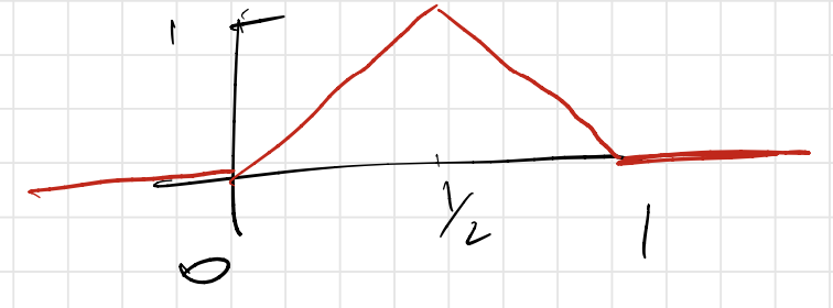
and then observe that:

What happens when we compose $m$ with itself several times? Define:

Then, we start seeing an actual sawtooth function. For example, for $L=2$, we see:

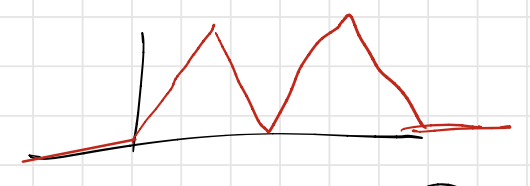
Iterating this $L$ times, we get a sawtooth that oscillates a bunch of times over the interval $[0,1]$ and is zero outside⁹. In fact, for any $L$, an easy induction will show that there will be $2^{L-1}$ “triangles”, which are formed using $2^L$ pieces.

But we also can observe that $m(x)$ can be written in terms of ReLUs. Specifically, if $\psi$ is the ReLU activation then:

which is a tiny (width-3, depth-2) ReLU network. Therefore, $m^{(L)}(x)$ is a univariate function that is exactly written out as width-3, depth-$2L$ ReLU network for any $L$.

Remark One can view $m^{(L)}(x)$ as a “bit-extractor” function since we have the property that $m^{(L)}(x) = m(\text{frac}(2^{L-1} x))$, where $\text{frac}(x) = x - \lfloor x \rfloor$ is the fractional part of any real number $x$. (Exercise: Prove this.) It is interesting that similar “bit-extractor” gadgets can be found in some earlier universal approximation proofs¹⁰.

So: we have constructed a neural network with depth $O(L)$ which simulates a piecewise linear function over the real line with $2^L$ pieces. In fact, this observation can be generalized quite significantly as follows.

Lemma If $p(x)$ and $q(x)$ are univariate functions defined over $[0,1]$ with $s$ and $t$ linear pieces respectively, then: (a) $\alpha p(x) + \beta q(x)$ has at most $s + t$ pieces over $[0,1]$. (b) $q(p(x))$ has at most $st$ pieces over $[0,1]$.

The proof of this lemma is an easy counting exercise over the number of “breakpoints” over $[0,1]$. Most relevant to our discussion, we immediately get the important corollary (somewhat informally stated here, there may be hidden constants which I am ignoring):

Corollary For any feedforward ReLU network $f$ with depth $\leq L$ and width $\leq 2^{L^\delta}$, then the total number of pieces in the range of $f$ is strictly smaller than $2^{L^2}$.

We are now ready for the proof of the main Theorem.

Proof Our target function $g$ will be the sawtooth function iterated $L^2 + 2$ times, i.e.,

Using Corollary we will show that that if $f$ is any feedforard ReLU net with depth $\leq L$ and sub-exponential width, then $f$ cannot approximate a significant fraction of the pieces in $g$. In terms of picture, let us consider the following figure:

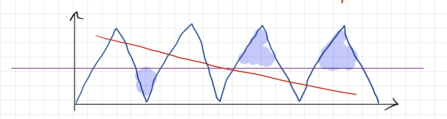
where $f$ is in red and $g$ (the target) is in navy blue. Let’s draw the horizontal line $y = 1/2$ in purple. We can count the total number of (tiny) triangles in $g$ to be (exactly) equal to

(the -1 is because the two edge cases have only a half-triangle each). Each of these tiny triangles have height 1/2, so their area is:

But any linear piece of $f$ has to have zero intersection at least half of these triangles (since this linear piece can either be above the purple line or below, not both). Therefore, if we look at the error restricted to this particular piece, the area under this curve should be at least the area of the missed triangles (shaded in blue). Therefore, the total error is lower bounded as follows:

This completes the proof.

Let us reflect a bit more on the above proof. The key ingredient was the fact that superpositions (adding units, essentially increasing the “width”) only have a polynomial increase on the number of pieces in the range of $g$, but compositions (essentially increasing the “depth”) have an exponential increase in the number of pieces.

But! this “hard” function $g$, which is the sawtooth over $[0,1]$, was very carefully constructed. To achieve the exponential scaling law in the number of pieces, the breakpoints in $g$ have to be exactly equispaced, and therefore the weights in every layer in the network have to be identical. Even a tiny perturbation to $g$ dramatically reduces the number of linear pieces in the range of the network. See the following figure illustrated in Hanin and Rolnick (2019)¹¹:

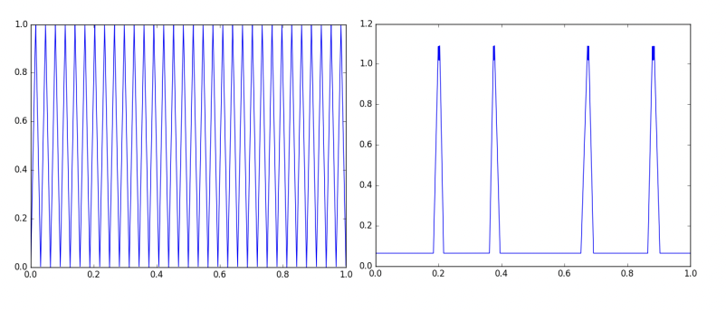
The plot on the left is the sawtooth function $g$, which, as we proved earlier, is representable via a depth-$O(L^2)$, width-3 ReLU net. The plot on the right is the function implemented by the same network as $g$ but with a tiny amount of noise added to its weights. So even when we did get a depth-separation result, it’s not at all “robust”.

All this to say: depth separation results for function approximation can be rather elusive; they seem to only exist for very special cases; and progress in this direction would result in several fundamental breakthroughs in complexity theory.

Depth and memorization

We will now turn to Approach 1. Let’s say that our goal was a bit more modest, and merely wanted to memorize a bunch of $n$ training data points with $d$ input features. Recall that we already showed that $O(\frac{n}{d})$ neurons are sufficient to memorize these points using a “peeling”-style proof.

Paraphrasing this fact: for depth-2 networks with $m$ hidden neurons, the memorization capacity is of the order of $d\cdot m$. This is roughly the same as the number of parameters in the network, so parameter counting intuitively tells us that we cannot do much better. What does depth $>2$ give us really?

Several recent (very nice) papers have addressed this question. Let us start with the following result by Yun et al.¹².

Theorem Let $X = \lbrace (x_i, y_i)_{i=1}^N \rbrace \subset \R^d \times \R$ be a dataset with distinct $x_i$ and $y_i \in [-1,1]$. Then, there exists a depth-3 ReLU network with hidden units $d_1, d_2$ where:

that exactly memorizes $X$.

The proof is somewhat involved, so we will give a brief sketch at the bottom of this page. But let us first study several implications of this result. First, we get the following corollary:

Corollary (Informal) A depth-3 ReLU network with width $d_1 = d_2 = O(\sqrt{N})$ is sufficient to memorize $N$ points.

This indicates a concrete separation in terms of memorization capacity between depth-2 and depth-3 networks. Suppose we focus on the regime where $d \ll N$. For this case, we have achieved a polynomial reduction in the number of hidden neurons in the network from $O(N)$ in the depth-2 case to $O(\sqrt{N})$ in the depth-3 case.

Notice that the number of parameters in the network still remains $\Theta(N)$ (and the condition in the above Theorem ensures this, since the “middle” layer has $d_1 \cdot d_2 \gtrsim N$ connections.) But there are ancillary benefits in reducing the number of neurons themselves (for example, in the context of hardware implementation) which we won’t get into.

Remark A similar result on memorization capacity can be obtained for situations with multiple labels (e.g. in the multi-class classification setting). If the dimension of the label is $d_y > 1$, then the condition is that $d_1 d_2 \gtrsim N d_y$.

Remark The multi-label case can be directly applied to provide width-lower bounds on memorizing popular datasets. For example, the well-known ImageNet dataset has about 10M image samples and performs classification over 1000 classes. The width bound suggests that we need networks of width no smaller than $\sqrt{10^7 \times 10^3} \approx 10^5$ ReLUs.

Yun et al.¹² also obtain a version of their result for depth-$L$ networks:

Theorem Suppose a depth-$L$ ReLU network has widths of hidden layers $d_1, d_2, \ldots, d_L$ then its memorization capacity is lower bounded by:

i.e., a network with this architecture can be tuned to memorize any dataset with at most $N$ points.

This result, while holding for general $L$-hidden-layer networks, doesn’t unfortunately paint a full picture; the proof starts with the result for $L = 2$, and then proceeds to show that all labels can be successively memorized “layer-by-layer”. In particular, to memorize $N$ data points, the width requirement remains $O(\sqrt{N})$ and it is not entirely clear if depth plays a role. We will come back to this shortly.

Several interesting questions arise. First, tightness. The above Theorem shows that depth-2, width-$\sqrt{N}$ networks are sufficient to memorize training sets of size $N$. But is this width dependence of $\sqrt{N}$ also necessary? Parameter counting suggests that this is indeed the case. Formally, Yun et al.¹² provide an elegant proof for a (matching) lower bound:

Theorem Suppose a depth-$3$ ReLU network has widths of hidden layers $d_1, d_2$. If

then there exists a dataset with $N$ points that cannot be memorized.

Proof (Complete).

Observe that this does not directly give lower bounds on the number of parameters needed to memorize data. We will come back to this question below.

Next, extensions to other networks. The above results are for feedforward ReLU networks; Yun et al.¹² also showed this for “hard-tanh” activations (which is a “clipped” ReLU activation that saturates at +1 for $x \geq 1$). Similar results (with number of connections approximately equal to the number of data points) have been obtained for polynomial networks¹³ and residual networks¹⁴.

What about more exotic families of networks? Could it be that there is some yet-undiscovered model that may give better memorization?

In a very nice (and surprisingly general) result, Vershynin¹⁵ showed the following:

Theorem (Informal) Consider well-separated data of unit norm and binary labels. Consider depth-$L$ networks ($L \geq 3$) with arbitrary activations across neurons but without exponentially narrow bottlenecks. If the number of “wires” in the second layer of a network and later:

is slightly larger than $N$, specifically:

then some choice of weights can memorize this dataset.

The high level idea in the proof of this result is to use the first layer as a preconditioner that separates data points into an almost-orthogonal set (in fact, a simple random Gaussian projection layer will do), and then any sequence of final layers that will memorize label assignments.

The precise definitions of “well-separatedness” and “bottlenecks” can be found in the paper, but the key here is that this bound is independent of depth, choice of activations (whether ReLU or threshold or some mixture of both), and any other architectural details. Again, we see that there doesn’t seem to be a clear impact of the depth parameter $L$ on network capacity.

For a more precise discussion along these lines, see the review section of a very nice (and recent) paper by Rajput et al.¹⁶.

Depth versus number of parameters

In the above discussion we saw that that moving from depth-2 to depth-3 networks helped significantly reduced the number of neurons needed to memorize $N$ arbitrary data points from $O(N)$ to $O(\sqrt{N})$ in several cases. The number of parameters in all these constructions remained $O(N)$ (but no better).

Is this the best possible we can do, or does depth help? We already encountered the result by Sontag¹⁷ showing an $\Omega(N)$ lower bound; specifically, given any network with sub-linear ($o(N)$) parameters, there exists at least one “worst-case” dataset that cannot be memorized.

Maybe our definition of memorization is too pessimistic, and we don’t have to fret about worst case behavior? Let us contrast Sontag’s result with other lower bounds from learning theory. Until now, we have quantified the memorization capacity of a network in terms of its ability to exactly interpolate any dataset. But we can weaken this definition a bit.

The VC-dimension of any family of models is defined as the maximum number of data points that the model can “shatter” (i.e., exactly interpolate labels). Notice that this is a “best-case” definition; if the VC dimension is $N$ there should exist at least one dataset of $N$ points (with arbitrary labels) that the network is able to memorize.

Existing VC dimension bounds state that if a network architecture has $W$ weights then the VC dimension is no greater than $O(W^2)$¹⁸ no matter the depth. Therefore, in the “best-case” scenario, to memorize $N$ samples with arbitrary labels, we would require at least $\Omega(\sqrt{N})$ parameters, and we could not really hope to do any better¹⁹.

Can we reconcile this gap between the “best” and “worst” cases of memorization capacity? In a very recent result, Vardi et al.⁵ have been able to show that the $\sqrt{N}$ dependence is in fact tight (up to log factors). Under the assumption that the data is bounded norm and well-separated, then a width-12, depth-$\tilde{O}(\sqrt{N})$ network with $\tilde{O}(\sqrt{N})$ parameters can memorize any dataset. This result improves upon a previous result²⁰ that had initially achieved a sub-linear upper bound of $O(N^{\frac{2}{3}})$ parameters.

The proof of this result is somewhat combinatorial in nature. We see (again!) the bit-extractor gadget network being used here. There is another catch: the bit complexity of the network is very large (it scales as $\sqrt{N}$), so the price to pay for a very small number of weights is that we end up stuffing many more bits in each weight.

Proof of 3-layer memorization capacity

(COMPLETE)