ECE-GY 6143, Spring 2020

Neural Network Architectures

Thus far, we have introduced neural networks in a fairly generic manner (layers of neurons, with learnable weights and biases, concatenated in a feed-forward manner). We have also seen how such networks can serve very powerful representations, and can be used to solve problems such as image classification.

The picture we have for our network looks something like this:

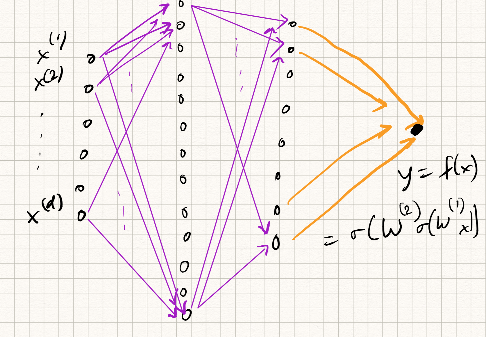
There are a few issues with this picture, however.

The first issue is computational cost. Let us assume a simple two layer architecture which takes a 400x400 pixel RGB image as input, has 1000 hidden neurons, and does 10-class classification. The number of trainable parameters is nearly 500 million. (Imagine now doing this calculation for very deep networks.) For most reasonable architectures, the number of parameters in the network roughly scales as $O(\tilde{d}^2 L)$, where $\tilde{d}$ is the maximum width of the network and $L$ is the number of layers. The quadratic scaling poses a major computational bottleneck.

This also poses a major sample complexity bottleneck – more parameters (typically) mean that we need a larger training dataset. But until about a decade ago, datasets with hundreds of millions (or billions) of training samples simply weren’t available for any application.

The second issue is loss of context. In applications such as image classification, the input features are spatial pixel intensities. But what if the image shifts a little? The classifier should still perform well (after all, the content of the image didn’t change). But fully connected neural networks don’t quite handle this well – recall that we simply flattened the image into a vector before feeding as input, so spatial information was lost.

A similar issue occurs in applications such as audio/speech, or NLP. Vectorizing the input leads to loss of temporal correlations, and general fully connected nets don’t have a mechanism to capture temporal concepts.

The third issue is confounding features. Most of our toy examples thus far have been on carefully curated image datasets (such as MNIST, or FashionMNIST) with exactly one object per image. But the real world is full of unpredictable phenomena (there could be occlusions, or background clutter, or strange illuminations). We simply will not have enough training data to robustify our network to all such variations.

Convolutional neural networks (CNNs)

Fortunately, we can resolve some of the above issues by being a bit more careful with the design of the network architecture. We focus on object detection in image data for now (although the ideas also apply to other domains, such as audio). The two Guiding Principles are as follows:

• Locality: neural net classifiers should look at local regions in an image, without too much regard to what is happening elsewhere.

• Shift invariance: neural net classifiers should have similar responses to the same object no matter where it appears in the image.

Both of these can be realized by defining a new type of neural net architecture, which is composed of convolution layers.

Definition

A quick recap of convolution from signal processing. We have two signals (for our purposes, everything is in discrete-time, so they can be thought of as arrays) $x[t]$ and $w[t]$. Here, $x$ will be called the input and $w$ will be called the filter or kernel (not to be confused with kernel methods). The convolution of $x$ and $w$, denoted by the operation $\star$, is defined as:

\[(x \star w)[t] = \sum_\tau x[t - \tau] w[\tau] .\]

It is not too hard to prove that the summation indices can be reversed but the operation remains the same:

\[(x \star w)[t] = \sum_\tau x[\tau] w[t - \tau] .\]

In the first sense, we can think of the output of the convolution operation as “translate-and-scale”, i.e., shifting various copies of $x$ by different amounts $\tau$, scaling by $w[\tau]$ and summing up. In the second sense, we can think of it as “flip-and-dot”, i.e., flipping $w$ about the $t=0$ axis, shifting by $t$ and taking the dot product with respect to $x$.

This definition extends to 2D images, except with two (spatial) indices:

\[(x \star w)[s,t] = \sum_\sigma \sum_\tau x[s - \sigma, t - \tau], w[\sigma, \tau]\]

Convolution has lots of nice properties (one can prove that convolution is linear, associative, and commutative). But the main property of convolution we will leverage is that it is equivariant with respect to shifts: if the input $x$ is shifted by some amount in space/time, then the output $x \star w$ is shifted by the same amount. This addresses Principle 2 above.

Moreover, we can also address Principle 1: if we limit the support (or the number of nonzero entries) of $w$, then this has the effect that the outputs only depend on local spatial (or temporal) behaviors in $x$!

[Aside: The use of convolution in signal/image processing is not new: convolutions are used to implement things like low-pass filters (which smooth the input) or high-pass filters (which sharpen the input). Composing a high-pass filter with a step-nonlinearity, for example, gives a way to locate sharp regions such as edges in an image. The innovation here is that the filters are treated as learnable from data].

Convolution layers

We can use the above properties to define convolution layers. Somewhat confusingly, the “flip” in “flip-and-dot” is ignored; we don’t flip the filter and hence use a $+$ instead of a $-$ in the indices:

\[z[s,t] = (x \star w)[s,t] = \sum_{\sigma = -\Delta}^{\Delta} \sum_{\tau = -\Delta}^{\Delta} x[s + \sigma,t + \tau] w[\sigma,\tau].\]

So, basically like the definition convolution in signal processing but with slightly different notation – so this is only a cosmetic change. The support of $w$ ranges from $-\Delta$ to $-\Delta$. This induces a corresponding region in the domain of $x$ that influences the outputs, which is called the receptive field. We can also choose to apply a nonlinearity $\phi$ to each output:

\[h[s,t] = \phi(z[s,t]).\]

The corresponding transformation is called feature map. The new picture we have for our convolution layer looks something like this:

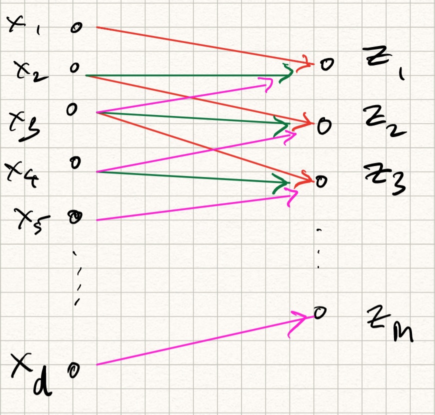
Observe that this operation can be implemented by matrix multiplication with a set of weights followed by a nonlinear activation function, similar to regular neural networks – except that there are two differences:

• Instead of being fully connected, each output coefficient is only dependent on $(2\Delta+1 \times 2\Delta+1)$-subset of input values; therefore, the layer is sparsely connected.

• Because of the shift invariance property, the weights of different output neurons are the same (notice that in the summation, the indices in $w$ are independent of $s,t$). Therefore, the weights are shared.

The above definition computed a single feature map on a 2D input. However, similar to defining multiple hidden neurons, we can extend this to multiple feature maps operating on multiple input channels (the input channels can be, for example, RGB channels of an image, or the output features of other convolution layers). So in general, if we have $D$ input channels and $F$ output feature maps, we can define:

\[\begin{aligned} z_i &= \sum_j x_j \star w_{ij} \\ h_i &= \phi(z_i). \end{aligned}\]

Combining the above properties means that the number of free learnable parameters in this layer is merely $O(\Delta^2 \times D \times F)$. Note that the dimension of the input does not appear at all, and the quadratic dependence is merely on the filter size! So if we use a $5 \times 5$ filter with (say) 20 input feature maps and 10 output feature maps, the number of learnable weights is merely $5000$, which is several orders of magnitude lower than fully connected networks!

A couple of more practical considerations:

• Padding: if you have encountered discrete-time convolution before, you will know that we need to be careful at the boundaries, and that the sizes of the input/output may differ. This is taken care of by appropriate zero-padding at the boundaries.

• Strides: we can choose to subsample our output in case the sizes are too big. This can be done by merely retaining every alternate (or every third, or every fourth..) output index. This is called stride length. [The default is to compute all output values, which is called a stride length of 1.]

• Pooling: Another way to reduce output size is to aggregate output values within a small spatial or temporal region. Such an aggregation can be performed by computing the mean of outputs within a window (average pooling), or computing the maximum (max pooling). This also has the advantage that the outputs become robust to small shifts in the input.

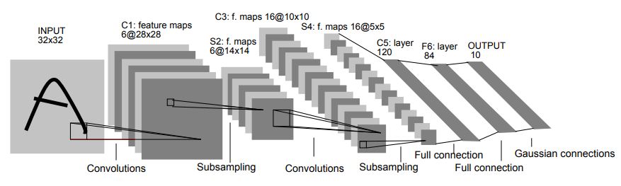
So there you have it: all the ingredients of a convolutional network. One of the first success stories of ConvNets was called LeNet, invented by LeCun-Bottou-Bengio-Haffner in 1998, which has the following architecture:

From 1998 to approximately 2015, most of the major advances in object detection were made using a series of successively deeper convolutional networks:

• AlexNet (2012), which arguably kickstarted the reemergence of neural nets in real-world applications. This resembled LeNet but with more feature maps and layers.

• VGGNet (2014), also similar but even bigger.

• GoogleNet (2014): this was an all-convolutional network (no fully connected layers anywhere, except the final classification).

After 2015, deeper networks were constructed using residual blocks, which we will only briefly touch upon below.

Training a CNN

Note that we haven’t talked about a separate algorithm for training a CNN. That is because we don’t need to: the backpropagation algorithm discussed in the previous lecture works very well! The computation graph is a bit different. Also, the weights are shared, so we need to be a bit more careful while deriving the backward pass rules. We won’t derive it again here; most deep learning software packages implement this under the hood.

Recurrent neural networks (RNNs)

Let us now turn our attention to a different set of applications. Consider natural language processing (NLP), where the goal might be to:

• perform document retrieval: we have already done this before;

• convert speech (audio waveforms) to text: used in Siri, or Google Assistant;

• achieve language translation: used in Google Translate,

• map video to text: used in automatic captioning,

among a host of other applications.

If we think of a speech signal or a sentence in vector/array form, notice that the contents of the vector exhibits both short range as well as long-range dependencies; for example, the start of a sentence may have relevance to the end of a sentence. (Example: “The cow, in its full glory, jumped over the moon” – the subject and object are at two opposite ends of the sentence.)

Classically, the tools to solve NLP problems were Markov models. If we assume a sequence of words $w = (w_1,w_2,\ldots,w_d)$, and define a probability distribution $P(w)$, then, short-range dependences could be captured via the Markov assumption that the likelihood of each word only depended on the previous word in the sentence:

\[P(w) = P((w_1,w_2,\ldots,w_d)) = P(w_1) \cdot P(w_2 | w_1) \cdot \ldots P(w_d | w_{d-1}) .\]

If we were being brave, we could extend it to two, or three, previous words – but realize that as we introduce more and more dependencies across time, the probability calculations quickly become combinatorially large.

Definition

An elegant way to resolve this issue and introduce long(er) range dependencies is via feedback. Thus far, we have strictly used feedforward connections, which are somewhat limiting in the case of NLP.

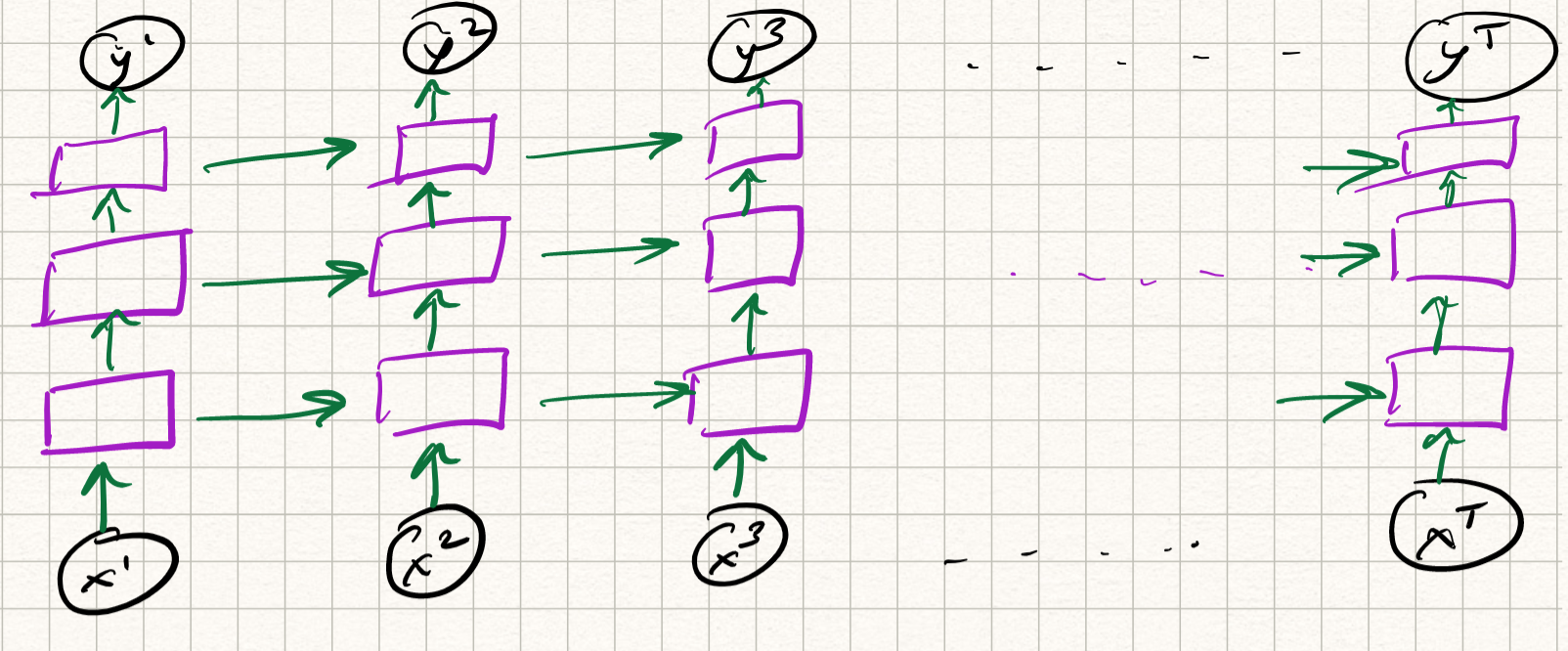
Let us now introduce a new type of neural net with self-loops which acts on time series, called the recurrent neural net (RNN). In reality, the self-loops in the hidden neurons are computed with unit-delay, which really means that the output of the hidden unit at a given time step depends both on the input at that time step, and the output at a previous time step. The mathematical definition of the operations are as follows:

\[\begin{aligned} h^{t} &= \phi(U x^{t} + W h^{t-1}) \\ y^{t} &= V h^{t} . \end{aligned}\]

So, historical information is stored in the output of the hidden neurons, across different time steps. We can visualize the flow of information across time by “unrolling” the network across time.

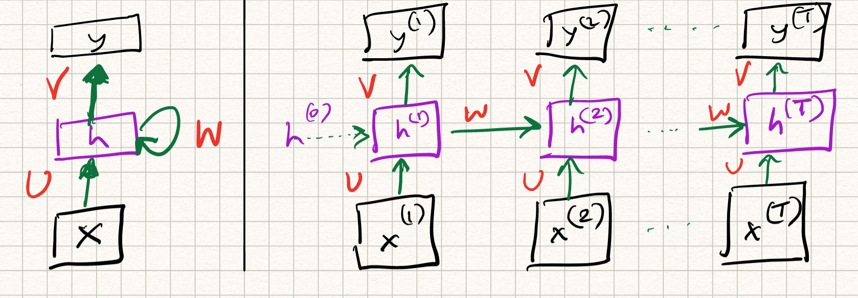
Observe that the layer weights $U, W, V$ are constant over different time steps; they do not vary. Therefore, the RNN can be viewed as a special case of deep neural nets with weight sharing.

Training an RNN

Again, training an RNN can be done using the same tools as we have discussed before: variants of gradient descent via backpropagation. The twist in this case is the feedback loop, which complicates matters. To simplify this, we simply unroll the feedback loop into $T$ time steps, and perform backpropagation through time for this unrolled (deep) network. There is considerable weight sharing here (since all the time instants have the same weight matrices), so we need to be careful when we apply the multivariate chain rules while computing the backward pass. But really it is all about careful book-keeping; conceptually the algorithm is the same.

Variations

RNNs are very powerful examples of the flexibility of neural nets. Moreover, the above example is for a single-layer RNN (which itself – let us be clear — is a deep network, if we imagine the RNN to be unrolled over time). We could make it more complex, and define a multi-layer RNN by computing the mapping from input to state itself via several layers. The equations are messy to write down so let’s just draw a picture:

Depending on how we define the structure of the intermediate layers, we get various flavors of RNNs:

• Gated Recurrent Units (GRU) networks
• Long Short-Term Memory (LSTM) networks
• Bidirectional RNNs
• Attention networks

and many others. An in-depth discussion of all these networks is unfortunately beyond the scope of this course.

Generalization in neural nets

Modern machine learning models (such as neural nets) typically have lots of parameters. For example, the best architecture as of the end of 2019 for object recognition, measured using the popular ImageNet benchmark dataset, contains 928 million learnable parameters. This is far greater than the number of training samples (about 14 million).

This, of course, should be concerning from a model generalization standpoint. Recall that we had previously discussed the bias-versus variance issue in ML models. As the number of parameters increases, the bias decreases (because we have more tunable knobs to fit our data), but the variance increases (because there is greater amount of overfitting). We get a curve like this:

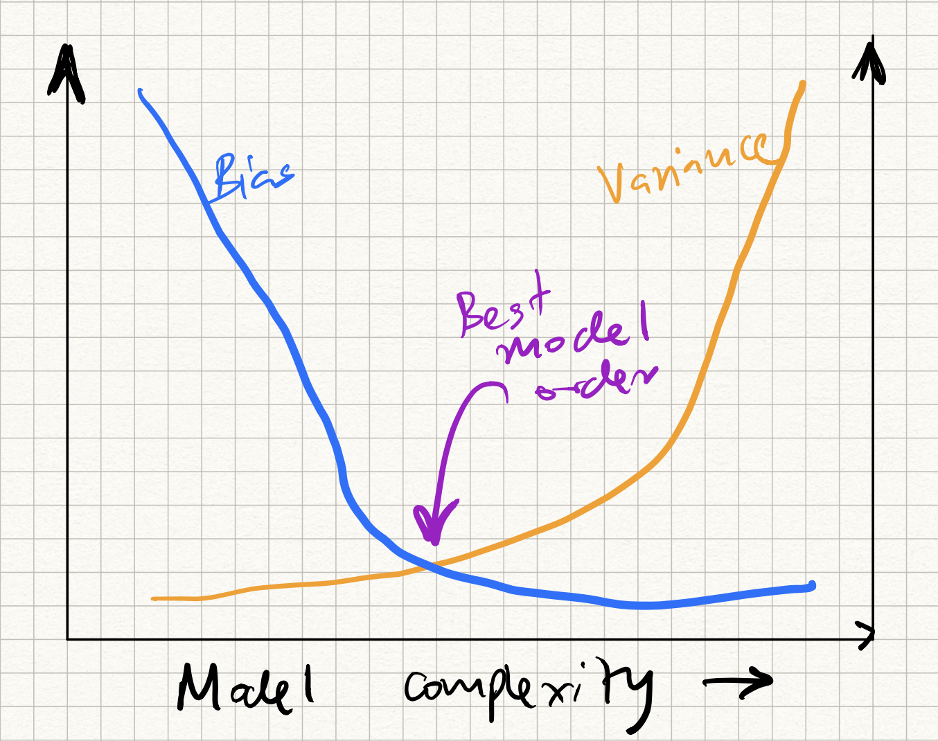
The question, then, is how to control the position on this curve so that we hit the sweet spot in the middle?

(It turns out that deep neural nets don’t quite obey this curve – a puzzling phenomenon called “double descent” occurs, but let us not dive too deep into it here; Google it if you are interested.)

We had previously introduced regularizers as a way to mitigate shortage of training samples, and in neural nets a broader class of regularization strategies exist. Simple techniques such as adding an extra regularizer do not work in isolation, and a few extra tricks are required. These include:

• Designing “bottlenecks” in network architecture: One way to regularize performance is to add a linear layer of neurons that is “narrower” than the layer preceding and succeeding it. We will talk about unsupervised learning below, and interpret this in the context of PCA.

• Early stopping: We monitor our training and validation error curves during the learning process. We expect training error to (generally) decrease, and validation error to flatten out (or even start increasing). The gap between the two curves indicates generalization performance, and we stop training when this gap is minimized. The problem with this approach is that if we train using stochastic methods (such as SGD) the error curves can fluctuate quite a bit and early stopping may lead to sub-optimal results.

• Weight decay: This involves adding an L2-regularizer to the standard neural net training loss.

• Dataset augmentation: To resolve the imbalance between the number of model parameters and the number of training examples, we can try to increase dataset size. One way to simulate an increased dataset size is by artificially transforming an input training sample (e.g. if we are dealing with images, we can shift, rotate, flip, crop, shear, or distort the training image example) before using it to update the model weights. There are smarter ways of doing dataset augmentation depending on the application, and libraries such as PyTorch have inbuilt routines for doing this.

• Dropout: A different way to solve the above imbalance is to simulate a smaller model. This can be (heuristically) achieved via a technique called dropout. The idea is that at the start of each iteration, we introduce stochastic binary variables called masks – $m_i$ – for each neuron. These random variables are 1 with probability $p$ and 0 with probability $1-p$. Then, in the forward pass, we “drop” individual neurons by masking their activations:

\[h_i = m_i \phi(z_i)\]

and in the backward pass, we similarly mask the corresponding gradients with $m_i$:

\[\partial_{z_i} \mathcal{L} = \partial_{h_i} \mathcal{L} \cdot m_i \cdot \partial_{z_i} \phi (z_i) .\]

During test time, all weights are scaled with $p$ in order to match expected values.

• Transfer learning: Yet another way to resolve the issue of small training datasets is to transfer knowledge from a different learning problem. For example, suppose we are given the task of learning a classifier for medical images (say, CT or X-Ray). Medical images are expensive to obtain, and training very deep neural networks on realistic dataset sizes may be infeasible. However, we could first learn a different neural network for a different task (say, standard object recognition) and finetune this network with the given available medical image data. The high level idea is that there may be common learned features across datasets, and we may not depend on re-learning all of them for each new task.