ECE-GY 6143

Model selection, bias-variance tradeoffs

OK, let’s hit a slight pause on the algorithms side. We have already seen 3 different algorithms to compute linear models for a given training dataset (matrix inversion, gradient descent, SGD). But why limit ourselves to linear models? Despite the benefits of linearity (easy to interpret, easy to compute, etc.) sometimes they may not always make sense:

We assumed that the data matrix is full-rank, which is necessary if the matrix inverse in linear regression has to exist. This is true in general only when the number of training data points ($n$) is greater than the dimension ($d$). If we have fewer data points than dimensions, the inverse may not exist, and the problem is ill-posed with many competing solutions. In general, having more parameters than training samples is a perilous situation, since any dataset can be fit using a linear model. This leads to unnecessarily high generalization error, which we discuss below. Therefore, the linear model may not be the right one to choose.
More generally, we assumed that all the data attributes (or features) are meaningful. For example, if we are to predict likelihood of diabetes of an individual from a whole bunch of physiological measurements (height, weight, eye color, blood sugar levels, Sp02, retinal measurements, age, lipid levels, WBC counts, etc.) it is likely that only a few attributes actually are useful in making a prediction. The catch, of course, is that a priori we do not know which features are the most important ones. The same with predicting likelihood of an email being spam or not using word counts. While not all words contribute to the “spamminess” of a message, certain special words (which constitute a small subset of the English language) tend to give it away.
We assumed that the data/labels intrinsically obey a linear relationship. But there is no reason that should be the case! In general, we need methods to learn more general nonlinear relationships in data.

The last point (nonlinear models) we will deal with when we discuss more sophisticated learning models such as kernel methods and neural nets. But one easy hack is to engineer lots of features from the data: given a data point $x$, we can compute any number of simple transformations ($x^2, x^3, \ldots, x^d, \ldots, 1/x, \ldots, \exp(-x), \ldots$), throw it all into an augmented dataset, and run linear regression on this new data. Of course, we run into the same issue as above: only a small subset of these features will be actually relevant to our problem, but we don’t a priori know which ones they are.

Let us tackle the first two aspects first (model selection). Until now, our setting has been the following. Given a training dataset ${x_i, y_i}$, fit a function $f$ such that $y_i \approx f(x_i)$. We assume that the data is sampled from a distribution $D$ that obeys an unknown but “true” relationship $y = t(x) + \epsilon$, where $\epsilon$ denotes irremovable i.i.d. zero-mean noise of variance $\sigma^2$.

But really, we care about performance on an unseen $x,y$. So even though we optimize training MSE in any regression problem, what we really care about is minimizing:

\[\text{Test MSE} = E_{(x,y)\sim D} (y - f(x))^2 .\]

where the expectation is over the draw of the training set and the noise.

We have no direct way to calculate this in reality (because the test set is not known beforehand). Therefore, while building ML models, this is typically simulated via a hold-out subset of the available training data, and pretending this is representative of the test-dataset. (In order to reduce simulation effects, this procedure is repeated $k$ times – given rise to the name k-fold cross validation).

So let us say we have estimated the test MSE, and we would like to reduce this number. What should we do next? One path forward is revealed by decomposing the test MSE into the following expectation (with respect to the choice of training set):

\[\begin{aligned} \text{Test MSE} &= E_{(x,y)\sim D} (y - f(x))^2 \\ &= E (t(x) + \epsilon - f(x))^2 \\ &= E (\epsilon)^2 + E [(t(x) - f(x))^2] \\ &= \sigma^2 + E(t(x) - f(x))^2 + \text{Var}(t(x) - f(x)) \\ &= \sigma^2 + \text{Bias}^2 + \text{Variance} \end{aligned}\]

where $\text{Bias}$ and $\text{Variance}$ are referring to the random variable $t(x) - f(x)$. For a more comprehensive derivation, see the treatment in Bishop’s textbook, Section 3.

Therefore, our MSE can be decomposed into three terms:

Irreducible noise $\sigma^2$: nothing can be done about this.
Bias of $f(x) - t(x)$: high bias typically corresponds to under-fitting, meaning that that $f$ does not express $t$ very well.
Variance of $f(x) - t(x)$: high variance typically corresponds to over-fitting, meaning that there is a lot of variation across difference draws of training sets.

This gives us a thumb rule to decide which model to select:

attempt to decrease bias/underfitting, so want more “complex” $f$
attempt to decrease variance/overfitting, so want “simpler” $f$

This has been classically been cast in terms of the following picture, called the bias-variance tradeoff curve:

Bias-variance tradeoff

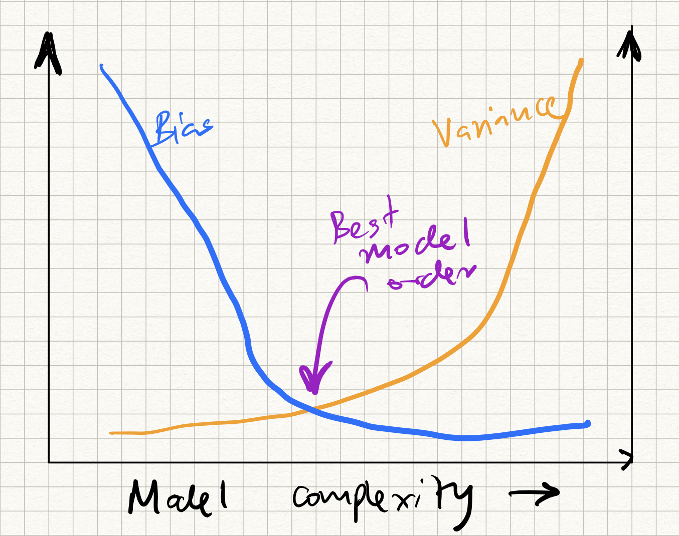
which we will experimentally demonstrate in class.

[Aside: an interesting new development is that modern ML methods such as deep neural nets do not seem to obey this simple tradeoff, but an analysis of why this happens is out of scope of this course.]