ECE-GY 6143, Spring 2020

Neural Networks

We have already introduced (single- and multi-layer) perceptrons in the previous lecture, and have interpreted them as a generalization to kernel methods. Deep neural networks are generalizations of the same concept.

The high level idea is to imagine each machine learning model in the form of a computational graph that takes in the data as input and produces the predicted labels as output. For completeness, let us reproduce the graphs for linear- and logistic regression here.

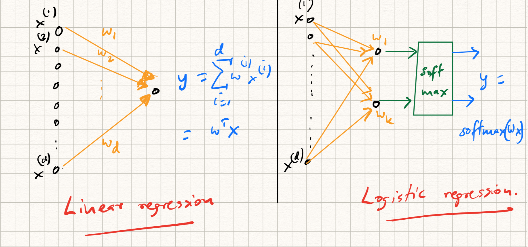
If we do that, we will notice that the graph in the above (linear) models has a natural feed-forward structure; these are instances of directed acyclic graphs, or DAG. The nodes in this DAG represent inputs and outputs; the edges represents the weights multiplying each input; outputs are calculated by summing up inputs in a weighted manner. The feed-forward structure represents the flow of information during test time; later, we will discuss instances of neural networks (such as recurrent neural networks) where there are feedback loops as well, but let us keep things simple here.

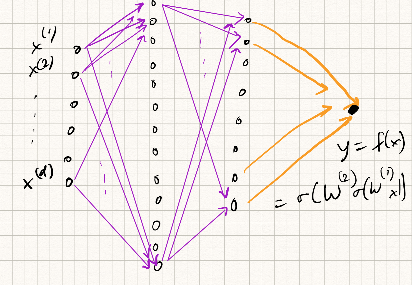
Let us retain the feed-forward structure, but now extend to a composition of lots of such units. The primitive operation for each “unit”, which we will call a neuron, will be written in the following functional form:

\[z = \sigma(\sum_{j} w_j x_j + b)\]

where $x_j$ are the inputs to the neuron, $w_j$ are the weights, $b$ is a scalar called the bias, and $\sigma$ is a nonlinear scalar transformation called the activation function. So linear regression is the special case where $\sigma(z) = z$, logistic regression is the special case where $\sigma(z) = 1/(1 + e^{-z})$, and the perceptron is the special case where $\sigma(z) = \text{sign}(z)$.

A neural network is a feedforward composition of several neurons, typically arranged in the form of layers. So if we imagine several neurons participating at the $l^{th}$ layer, we can stack up their weights (row-wise) in the form of a weight matrix $W^(l)$. The output of neurons forming each layer forms the corresponding input to all of the neurons in the next layer. So a 3-layer neural network would have the functional form:

\[\begin{aligned} z_1 &= \sigma^{1}(W^{1} x + b^{1}), \\ z_2 &= \sigma^{2}(W^{2} z_1 + b^{2}), \\ y &= \sigma^{3}(W^{3} z_2 + b^{3}) . \end{aligned}\]

Analogously, one can extend this definition to $L$ layers for any $L \geq 1$. The nomenclature is a bit funny sometimes. The above example is either called a “3-layer network” or “2-hidden-layer network”; the output $y$ is considered as its own layer and not considered as “hidden”.

Neural nets have a long history, dating back to the 1950s, and we will not have time to go over all of it. We also will not have time to go into biological connections (indeed, the name arises from collections of neurons found in the brain, although the analogy is somewhat imperfect since we don’t have a full understanding of how the brain processes information.)

The computational reason why neural nets are rather powerful is that they are “universal approximators”: a feed-forward network with a single hidden layer of finitely many neurons with suitably chosen weights can be used to approximate any continuous function. This works for a large range of activation functions. This property is called the Universal Approximation Theorem (UAT) and an early version can be attributed to Cybenko (1989). So for most prediction problems, if our goal is to learn an unknown prediction function $f$ for which $y = f(x)$, we can pretend that it can be approximated by a neural network, and learn its weights.

The problem, of course, is that while the UAT confirms the mere existence of a neural network as the solution for most learning problems, it does not address practical issues. Examining the theorem carefully indicates that even though we use just one hidden layer, we may need an exponentially large number of neurons even in moderate cases. So therefore, the UAT works for shallow, wide networks. To resolve this, the trend over the last decade has been to trade off between width and depth: namely, keep width manageable (typically, of similar size as the input) but concatenate multiple layers. (Hence the name “deep neural networks”, or “deep learning”).

Leaving beside theoretical considerations, one can identify several questions of practical

• How do we choose the widths, types, and number, of layers in a neural network?

• How do we learn the weights of the network?

• Even if the weights were somehow learned using a (large) training dataset, does the prediction function work for new examples?

The first question is a question of designing representation. The second is a question of choice of training algorithm. The third is an issue of generalization. Intense research has occurred (and is still ongoing) in all three questions.

Designing network architectures

In typical neural networks, each hidden layer is composed of identical units (i.e., all neurons have the same functional form and activation functions).

Activation functions of neurons are essential for modeling nonlinear trends in the data. (This is easy to see: if there were no activation functions, then the only kind of functions that neural nets could model were linear functions). Typical activation functions include:

• the sigmoid $\sigma(z) = 1/(1 + e^{-z})$.
• the hyperbolic tan $\sigma(z) = (1 - e^{-2z})/(1 + e^{-2z})$.
• the ReLU (rectified linear unit) $\sigma(z) = \max(0,z)$.
• the hard threshold $\sigma(z) = \text{step}(z)$.
• the sign function $\sigma(z) = \text{sign}(z)$.

among many others. The ReLU is most commonly used nowadays since it does not suffer from the vanishing gradients problem (notice that all the other activation functions flatten out for large values of $z$, which makes it difficult to calculate gradients.)

There are also various types for layers:

• Dense layers – these are basically layers of neurons whose weights are unconstrained

• Convolutional layers – these are layers of neurons whose weights correspond to filters that perform a (1D or 2D) convolution with respect to the input.

• Pooling layers – These act as “downsampling” operations that reduce the size of the output. There are many sub-options here as to how to do so.

• Batch normalization layers – these operations rescale the output after each layer by adjusting the means and variances for each training mini-batch.

• Recurrent layers – these involve feedback connections.

• Residual layers – there involve “skip connections” where the outputs of Layer $l$ connect directly to Layer $l+2$.

• Attention layers – these are used in NLP applications,

among many others.

As you can see, there are tons of ways to mix and match various architectural ingredients to come up with new networks. How do we decide which recipe to use for specific applications and datasets is an open question. Good practice indicates the following thumb rule: just use architectures that have known to work for other similar domain applications. We will examine a few in homework and labs.

Training algorithms

Let us assume that a network architecture (i.e., the functional form of the prediction function $f$) has been decided upon. How do we learn the parameters (i.e., the weights and biases) of the network?

Fortunately, the basic approach is similar to what we have seen before: we first choose a suitable loss function, and then use (variations) of gradient descent to optimize it. (For example, in a regression or classification setting, we might choose the cross-entropy loss.) Stack up all the weights and biases of the network into a variable $W$ Then, we first define:

\[L(W) = \sum_{i=1}^n l(y_i, f(x_i)) + \lambda R(W)\]

where $l(\cdot, \cdot)$ is the loss applied for a particular prediction and $R(\cdot)$ is an optional regularizer. Then, we train using GD (or more commonly, minibatch SGD):

\[W^{t+1} = W^{t} - \alpha^{t} \left( \sum_{i \in S} \nabla l(y_i, f_W(x_i)) + \lambda \nabla R(W) \right).\]

where $S$ is a minibatch of samples. So really, everything boils down to computing the gradient of the loss. As we will see below, this may become cumbersome.

A toy example

Let us work out the gradient of the ridge regression loss for a single neuron with a sigmoid activation with a single scalar data point. This is obviously the easiest example. The model is as follows:

\[\begin{aligned} z &= wx + b,~f(z) = \sigma(z),\\ L(w,b) &= 0.5 (y - \sigma(wx + b))^2 + \lambda w^2. \end{aligned}\]

Calculation of the gradient is basically an invocation of the chain rule from calculus:

\[\begin{aligned} \frac{\partial L}{\partial w} &= (\sigma(wx + b) - y) \sigma'(wx + b) x + 2 \lambda w, \\ \frac{\partial L}{\partial b} &= (\sigma(wx + b) - y) \sigma'(wx + b). \end{aligned}\]

Immediately, we notice some inefficiencies. First, the expressions are already very complicated (can you imagine how long the expressions will become for arbitrary neural nets?). Sitting and deriving gradients is tedious and may lead to errors.

Second, notice that the above gradient computations are redundant. We have computed $\sigma(wx + b)$ and $\sigma’(wx + b)$ twice, one each in the calculations of $\frac{\partial L}{\partial w}$ and $\frac{\partial L}{\partial b}$. Digging even deeper, the expression $wx + b$ appears four times. Is there a way to avoid repeatedly calculating the same expression?

The backpropagation algorithm

The intuition underlying the backpropagation algorithm (or backprop for short) is that we can solve both of the above issues by leveraging the structure of the network itself. Let us decompose the model a bit more clearly as follows:

\[\begin{aligned} z &= wx + b, \\ u &= \sigma(z), \\ l &= 0.5 (y-u)^2, \\ r &= w^2, \\ L &= l + \lambda r. \end{aligned}\]

This sequence of operations can be written in the form of the following computation graph:

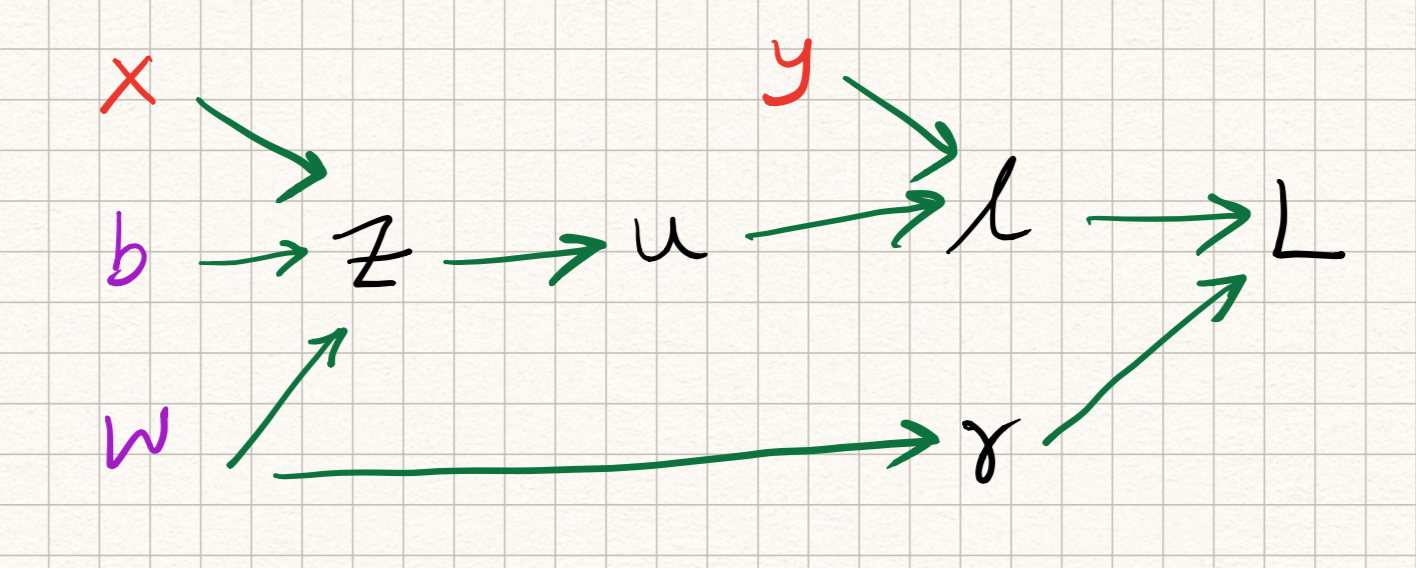
Observe that the computation of the loss $L$ can be implemented via a forward pass through this graph. The algorithm is as follows. If a computation graph $G$ has $N$ nodes, let $v_1, \ldots, v_N$ be the outputs of this graph (so that $L = v_N$).

function FORWARD():

1. for $i = 1, 2, \ldots, N$:

   a. Compute $v_i$ as a function of $\text{Parents}(v_i)$.

Now, observe (via the multivariate chain rule) that the gradients of the loss function with respect to the output at any node only depends on what variables the node influences (i.e., its children). Therefore, the gradient computation can be implemented via a backward pass through this graph.

function BACKWARD():

1. For $i = N-1, \ldots 1$:

   a. Compute \(\frac{\partial L}{\partial v_i} = \sum_{j \in \text{Children}(v_i)} \frac{\partial L}{\partial v_j} \frac{\partial v_j}{\partial v_i}\)

Maybe best to explain via example. Let us revisit the above single neuron case, but use the BACKWARD() algorithm to compute gradients of $L$ at each of the 7 variable nodes ($x$ and $y$ are inputs, not variables) in reverse order. Also, to abbreviate notation, let us denote $\partial_x f := \frac{\partial f}{\partial x}$.

We get:

\[\begin{aligned} \partial_L L &= 1, \\ \partial_r L &= \lambda, \\ \partial_l L &= 1, \\ \partial_u L &= \partial_l L \cdot \partial_u l = u-y, \\ {\partial_z L} &= {\partial_u L} \cdot {\partial_z u} = \partial_u L \cdot \sigma'(z), \\ {\partial_w L} &= {\partial_z L} \cdot {\partial_w z} + {\partial_r L} \cdot {\partial_w r} = \partial_u L \cdot x + \partial_r L \cdot 2 w, \\ {\partial_b L} &= {\partial_z L} \cdot {\partial_b z} = {\partial_z L}. \end{aligned}\]

Note that we got the same answers as before, but now there are several advantages:

• no more redundant computations: every partial derivative depends cleanly on partial derivatives on child nodes (so, operations that have already been computed before) and hence there is no need to repeat them.

• the computation is very structured, and everything can be calculated by traversing once through the graph.

• the procedure is modular, which means that changing (for example) the loss, or the architecture, does not change the algorithm! The expressions for $L$ changes but the procedure for computation remains the same.

In all likelihood, you will not have to implement backpropagation by hand in real applications: most neural net software packages (like PyTorch) include an automatic differentiation routine which implement the above operations efficiently. But under the hood, this is what is going on.