Chapter 4 - A primer on optimization

In the first few chapters, we covered several results related to the representation power of neural networks. We obtained estimates — sometimes tight ones — for the sizes of neural networks needed to memorize a given dataset, or to simulate a target prediction function.

However, most of our theoretical results used somewhat funny-looking constructions of neural networks. Our theoretically best-performing networks were all either too wide or too narrow, and didn’t really look like the typical deep networks that we see in practice.

But even setting aside the issue of size, none of the (theoretically attractive) techniques that we used to memorize datasets resemble deep learning practice. When folks refer to “training models”, they almost always are talking about fitting datasets to neural networks via local, greedy, first-order algorithms such as gradient descent (GD), or stochastic variations (like SGD), or accelerations (like Adam), or some other such approach.

In the next few chapters, we address the question:

Do practical approaches for model training work well?

This question is once again somewhat ill-posed, and we will have to be precise about what “work” and “well” mean in the above question. (From the practical perspective: an overwhelming amount of empirical evidence seems to suggest that they work just fine, as long as certain tricks/hacks are applied.)

While there is very large variation in the way we train deep networks, we will focus on a handful of the most canonical settings, analyze them, and derive precise bounds on their behavior. The hope is that such analysis can illuminate differences/tradeoffs between different choices and provide useful thumb rules for practice.

Setup

Most (all?) popular approaches in deep learning do the following:

• Write down the loss (or empirical risk) in terms of the training data points and the weights. (Usually the loss is decomposable across the data points). So if the data is $(x_i,y_i)_{i=1}^n$ then the loss looks something like:

  \[L(w) = \frac{1}{n} \sum_{i=1}^n l(y_i,\hat{y_i}), \quad \hat{y_i} = f_w(x_i),\]

  where $l(\cdot,\cdot) : \R \times \R \rightarrow \R_{\geq 0}$ is a non-negative measure of label fit, and $f_w$ is the function represented by the neural network with weight/bias parameters $w$. We are abusing notation here since we previously used $R$ for the risk, but let’s just use $L$ to denote loss.

• Then, we seek the weights/biases $w$ that optimize the loss:

  \[\hat{w} = \arg \min_w L(w) .\]

  Sometimes, we throw in an extra regularization term defined on $w$ for kicks, but let’s just stay simple for now.

• Importantly, invariably, the above optimization is carried out using a simple, iterative, first-order method. For example, if gradient descent (GD) is the method of choice, then discovering $\hat{w}$ amounts to iterating the following recursion:

  \[w \leftarrow w - \eta \nabla_w L(w)\]

  some number of times. Or, if SGD is the method of choice, then discovering $\hat{w}$ amounts to iterating the following recursion:

  \[w \leftarrow w - \eta g_w\]

  where $g_w$ is some (properly defined) stochastic approximation of $\nabla L(w)$. Or if Adam¹ is the method of choice, then discovering $\hat{w}$ amounts to iterating…a slightly more complicated recursion, but still a first-order method involving gradients and nothing more. You get the picture.

In this chapter, let us focus on GD and SGD. The following questions come to mind:

• Do GD and SGD converge at all.
• If so, do they converge to the set (or a set?) of globally optimal weights.
• How many steps do they need to converge reliably.
• How to pick step size, or (in the case of SGD) batch size, or other parameters.

among many others.

Before diving in to the details, let us qualitatively address the first couple of questions.

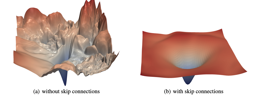
Intuition tells us that convergence in a local sense is to be expected, but converegence to global minimizers seems unlikely. Indeed, it is easy to prove that for anything beyond the simplest neural networks, the loss function $L(w)$ is extremely non-convex. Therefore the “loss landscape” of $L(w)$, viewed as a function of $w$, has many peaks, valleys, and ridges, and a myopic first-order approach such as GD may be very prone to get stuck in local optima, or saddle points, or other stationary points. A fantastic paper² by Xu et al. proposes creative ways of visualizing these high-dimensional landscapes.

Somewhat fascinatingly, however, it turns out that this intuition may not be correct. GD/SGD can be used to train models all the way down to zero train error (at least, this is common for deep networks used in classification.) This fact seems to have been folklore, but was systematically demonstrated in a series of interesting experiments by Zhang et al.³.

We will revisit this fact in the next two chapters. But for now, we limit ourselves to analyzing the local convergence behavior of GD/SGD. We establish the more modest claim:

(S)GD converges to (near) stationary points, provided $L(w)$ is smooth.

The last caveat — that $L(w)$ is required to be smooth — is actually a rather significant one, and excludes several widely used architectures used in practice. For example, the ubiquitous ReLU activation function, $\psi(z) = \max(z,0)$, is not smooth, and therefore neural networks involving ReLUs don’t lead to smooth losses.

This should not deter us. The analysis is still very interesting and useful; it is still applicable to other widely used architectures; and extensions to ReLUs can be achieved with a bit more technical heavy lifting (which we won’t cover here). For a more formal treatment of local convergence in networks with nonsmooth activations, see, for example, the paper by Ji and Telgarsky⁴, or these lecture notes⁵.

Gradient descent

We start with analyzing gradient descent for smooth loss functions. (As asides, we will also discuss application of our results to convex functions, but these functions are not common in deep learning and therefore not our focus.)

Let us first define smoothness. (All norms below refer to the 2-norm, and all gradients are with respect to the parameters.)

Definition $L$ is said to be $\beta$-smooth if $L$ has $\beta$-Lipschitz gradients:

With some algebra, one can arrive at the following lemma.

Lemma If $L$ is twice-differentiable and $\beta$-smooth, then the eigenvalues of its Hessian are less than $\beta$:

Equivalently, $L(w)$ is upper-bounded by a quadratic function:

for all $w,u$.

Basically, the smoothness condition (or its implications according to the above Lemma) says that if $\beta$ is not unreasonably big, then the gradients of $L(w)$ are rather well-behaved.

It is natural to see why something like this condition is needed to analyze GD. If smoothness did not hold and the gradient was not well-behaved, then first-order methods such as GD are not likely to be very informative.

There is a second natural reason why this definition is relevant to GD. Imagine, for a moment, not minimizing $L(w)$, but rather minimizing the upper bound:

This is a convex (in fact, quadratic) function of $w$. Therefore, it can be optimized very easily by setting $\nabla B(w)$ to zero and solving for $w$:

This is the same as a single step of gradient descent starting from $u$ (with step size inversely proportional to the smoothness parameter). In other words, gradient descent is nothing but the successive optimization of a Lipschitz upper bound of in every iteration⁶.

We are now ready to prove our first result.

Theorem If $L$ is $\beta$-smooth, then GD with fixed step size converges to stationary points.

Proof Consider any iteration of GD (with a step size $\eta$ which we will specify shortly):

This means that:

Plug this value of $w-u$ into the quadratic upper bound to get:

This inequality already gives a proof of convergence. Suppose that the step size is small enough such that $\eta < \frac{2}{\beta}$. We are in one of two situations:

1. Either $\nabla L(u) = 0$, in which case we are done — since $u$ is a stationary point.

2. Or $\nabla L(u) \neq 0$, in which case $\lVert \nabla L(u) \rVert > 0$ and the second term in the right hand side is strictly positive. Therefore GD makes progress (and decreases $L$ in the next step).

Since $L$ is lower bounded by 0 (since we have assumed a non-negative loss), we get convergence.

This argument does not quite tell us how many iterations are needed by GD. To estimate this, let us just set $\eta = \frac{1}{\beta}$. This choice is not precisely necessary to get similar bounds, but the algebra becomes simpler. Let’s just rename $w_i := u$ and $w_{i+1} := w$. Then, the last inequality becomes:

Telescoping from $w_0, w_1, \ldots, w_t$, we get:

(since $L_\text{opt}$ is the smallest achievable loss.) Therefore, if we pick $i = \arg \min_{i < t} \nabla \lVert L(w_i) \rVert^2$ as the estimate with lowest gradient norm and set $\hat{w} = w_{i}$, then we get:

which implies that if $L_0$ is bounded (i.e.: we start somewhere reasonable) then GD reaches a point $\hat{w}$ within at most $t$ iterations whose gradient norm is

at most. To put it a different way, to find an $\varepsilon$-stationary point, GD needs:

iterations.

Notice that the proof is simple: we didn’t use much information beyond the definition of Lipschitz smoothness. But it already reveals a lot.

First, step sizes in standard GD can be set to a constant. Later, we will analyze SGD (where step sizes have to be variable.)

Second, step sizes should be chosen inversely proportional to $\beta$. This makes intuitive sense: if $\beta$ is large then gradients are wiggling around, and therefore it is prudent to take small steps. On the other hand, it is not easy to estimate Lipschitz smoothness constants (particularly for neural networks), so in practice $\eta$ is just tuned by hand.

Third, we only get convergence in the “neighborhood” sense (in that there is some point along the trajectory which is close to the stationary point). It is harder to prove “last-iterate” convergence results. In fact, one can even show that GD can go near a stationary point, spend a very long time near this point, but then bounce away later⁷.

Fourth, we get $\frac{1}{\sqrt{t}}$ error after $t$ iterations. The terminology to describe this error rate is not very consistent in the optimization literature, but one might call this a “sub-linear” rate of convergence.

Let us now take a lengthy detour into classical optimization. What if $L$ were smooth and convex? As mentioned above, convex losses (as a function of the weights) are not common in deep learning; but it is instructive to understand how much convexity can buy us.

Life is much simpler now, since we can expect GD to find a global minimizer if $L$ is convex (i.e., not just a point where $\nabla L \approx 0$, but actually a point where $L \approx L_{\text{opt}}$).

How do we show this? While smoothness shows that $L$ is upper bounded by a quadratic function, convexity implies that $L$ is also lower bounded by tangents at every point. The picture looks like this:

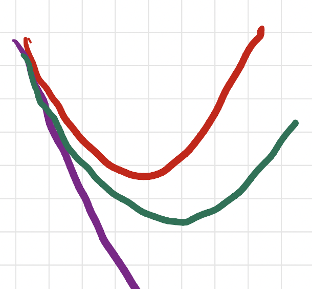
and mathematically, we have:

This lets us control not just $\nabla L$ but $L$ itself. Formally, we obtain:

Theorem If $L$ is $\beta$-smooth and convex, then GD with fixed step size converges to a minimizer.

Proof

Let $w^*$ be some minimizer, which achieves loss $L_{\text{opt}}$.

(Q. What if there is more than one minimizer? Good question!)

Set $\eta = \frac{1}{\beta}$, as before. We will bound the error in weight space as follows:

From the smoothness proof above, we already showed that

Moreover, plugging in $u = w_i$ and $w = w^*$ in the convexity lower bound, we get:

Therefore, we can bound both the rightmost terms in the weight error:

Therefore, we can invoke a similar argument as in the smoothness proof. One of two situations:

1. Either $L_{i+1} = L_{\text{opt}}$, which means we have achieved a point with optimal loss.

2. Or, $L_{i+1} > L_{\text{opt}}$, which means GD decreases weight error.

Therefore, we get convergence. In order to estimate the number of iterations, rearrange terms:

and telescope $i$ from 0 to $t-1$ to get:

which gives:

Therefore, the optimality gap decreases as $1/t$ and to find an $\varepsilon$-approximate point (assuming we start somewhere reasonable), GD needs $O(\frac{\beta}{\varepsilon})$ iterations.

Similar conclusions as above. Constant step size suffices for GD. Step size should be inversely proportional to smoothness constant. Convexity gives us a “last-iterate” bound, as well as parameter estimation guarantees.

Another aside: $L$ smooth and strongly convex? Then $L$ is both lower and upper bounded by quadratics. Therefore, optimization is easy; exponential ($e^{-t}$) rate of convergence. Fill this in.

So the hierarchy is as follows:

• GD assuming smoothness: $\frac{1}{\sqrt{t}}$ rate

• GD assuming smoothness + convexity: $\frac{1}{t}$ rate

• Momentum accelerated GD: $\frac{1}{t^2}$ rate. We won’t prove this; see the paper by Nesterov. Remarkably, this is the best possible one can do with first-order methods such as GD.

• GD assuming smoothness and strong convexity: $\exp(-t)$ rate .

The Polyak-Lojasiewicz (PL) condition

Above, we saw how leveraging smoothness, along with (strong) convexity, of the loss results in exponential convergence of GD. However (strong) convexity is not that relevant in the context of deep learning. This is because losses are very rarely convex in their parameters.

However, there is a different characterization of functions (other than convexity) that also implies fast convergence rates of GD. This property was introduced by Polyak⁸ in 1963, but has somehow not been very widely publicized. It was re-introduced to the ML optimization literature by Karimi et al.⁹ and its relevance (particularly in the context of deep learning) is slowly becoming apparent.

Definition A function $L$ (whose optimum is $L_{\text{opt}}$) is said to satisfy the Polyak-Lojasiewicz (PL) condition with parameter $\alpha$ if:

for all $u$ in its domain.

The reason for the “2” sitting before $\alpha$ will become clear. Intuitively, the PL condition says that if $L(u) \gg L_{\text{opt}}$ then $\lVert \nabla L(u) \rVert$ is also large. More precisely, the norm of the gradient at any point grows at least as the square root of the (functional) distance to the optimum.

Notice that there is no requirement of convexity in the definition of the PL condition. For example, the function:

has a plot that looks like

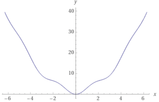
which is non-convex upon inspection, but nonetheless satisfies the PL condition with constant $\alpha = \frac{1}{32}$.

(However, the converse is true. Strong convexity implies the PL condition, but PL is far more general. We return to this in Chapter 6.)

We immediately get the following result.

Theorem If $L$ is $\beta$-smooth and satisfies the PL condition with parameter $\alpha$, then GD exponentially converges to the optimum.

Proof Follows trivially. Let $\eta = \frac{1}{\beta}$. Then

Plug $w_{t+1} - w_t$ into the smoothness upper bound. We get:

But since $L$ satisfies PL, we get:

Simplifying notation, we get:

which implies that GD converges at $\exp(-\frac{\alpha}{\beta}t)$ rate.

Why is the PL condition interesting? It has been shown that several neural net training problems satisfy PL.

1. Single neurons (with leaky ReLUs.)

2. Linear neural networks.

3. Linear residual networks (with square weight matrices).

4. Others? Wide networks? Complete.

Stochastic gradient descent (SGD)

We have obtained a reasonable picture of how GD works, how many iterations it needs, etc. But how does the picture change with inexact (stochastic) gradients?

This question is paramount in deep learning practice, since nobody really does full-batch GD. Datasets are massive, and since the loss is decomposable across all the data points, gradients of the loss require making a full sweep of the training dataset for each iteration, which no one really has time.

Even more so, it seems that stochastic gradients (instead of full gradients) may influences generalization behavior. Anecdotally, it was observed that models trained by SGD typically improved over models trained with full-batch gradient descent. Therefore, there may be some hidden benefit of stochasticity.

To explain this, there were a ton of papers discussing the distinction between “sharp” versus “flat” minima¹⁰, and how the latter type of minima generalize better, and how minibatch methods (such as SGD) favor flat minima, and therefore SGD gives better solutions period. Folks generally went along with this explanation. However, since this initial flurry of papers this common belief has since been somewhat upended.

First off, it is not really clear how “sharpness” or “flatness” should be formally defined. A paper by Dinh et al.¹¹ showed that good generalization can be obtained even if the model corresponds to a very “sharp” minimum in the loss landscape (for most commonly accepted definitions of “sharp”). So even if SGD finds flatter minima, it is unclear whether such minima are somehow inherently better.

A very recent paper by Geiping et al.¹² in fact finds the opposite; performance by GD (with properly tuned hyperparameters and regularization) matches that of SGD. Theory is silent on this matter and I am not aware of any concrete separation-type between GD and SGD for neural networks.

Still, independent of whether GD is theoretically better than SGD or not, it is instructive to analyze SGD (since everyone uses it.) Let us derive an analogous bound on the error rates of SGD.

In SGD, our updates look like:

Here $g_i$ is a noisy version to the full gradient $\nabla L(w_i)$ (where the “noise” here is due to minibatch sampling). Due to stochasticity, $g_i$ (and therefore, $w_i$) are random variables, and we should analyze convergence in terms of their expected value.

Intuitively, meaningful progress is possible only when the noise variance is not too large; this is achieved if the minibatch size is not too small. The following assumptions are somewhat standard (although rigorously proving this takes some effort.)

Property 1: Unbiased gradients: We will assume that in expectation, $g_i$ is an unbiased estimate of the true gradient. In other words, if $\varepsilon_i = g_i - \nabla L(w_i)$, then

Property 2: Bounded gradients: We will assume that the gradients are uniformly bounded in magnitude by a constant:

Remark Property 1 is fine if we sample the terms in the gradient uniformly at random. Property 2 is hard to justify in practice. (In fact, for convex functions this is not even true!) But better proofs such as this¹³ and this¹⁴ have shown that similar rates of convergence for SGD are possible even if we relax this assumption, so let’s just go with this for now and assume it can be fixed.

Assuming the above two properties, we will prove:

Theorem If $L$ is $\beta$-smooth, then SGD converges (in expectation) to an $\varepsilon$-approximate critical point in $O\left(\frac{\beta}{\varepsilon^4}\right)$ steps.

Proof Let’s run SGD with fixed step-size $\eta$ for $t$ steps. From the smoothness upper bound, we get:

But $w_{t+1} - w_t = - \eta g_t$. Plugging into the above bound and rearranging terms:

Take expectation on both sides. Property 1 and 2 give us:

Telescope from 0 through $T$, and divide by $\eta T$. Then we get:

This is true for all $\eta$. In order to get the tightest upper bound and minimize the right hand side, we need to balance the two terms on the right. This is achieved if:

Plugging this in, ignoring all other constants, we get:

This concludes the proof.

Hierarchy:

• SGD assuming Lipschitz smoothness: $\frac{1}{t^{1/4}}$

• SGD assuming Lipschitz smoothness + convexity: $\frac{1}{\sqrt{t}}$

Other rates?

Extensions

• Nesterov momemtum

(COMPLETE).