Lecture 3: Deep Neural Nets

In which we encounter deep neural networks, their challenges, and how to fix them.

Learning Deep Networks: Tips and Tricks

In the previous lecture, we showed how to perform efficient gradient-descent style updates for learning the weights of deep neural networks. At a high level, the approach was to do the following:

• formulate the network architecture, clearly specifying the trainable parameters (i.e., the weights and biases)
• write down a suitable loss function in terms of the weights/biases and the training data
• update the weights using the backpropagation algorithm, which consists of two stages in each minibatch iteration:
  • a forward pass through the network that computes the outputs for all neurons using the current set of weights:
  • a backward pass through the network that computes the gradient of the loss function with respect to the weights using the chain rule for vector derivatives.

The feedforward structure of a (standard) deep neural network enables both forward and backward passes to be done efficiently (i.e., in running time that is linear in the number of parameters).

Let us deconstruct the training process a bit more in detail. Along the way we will discover (and solve) many issues of practical importance: how to properly set up the training; how to improve upon gradient descent; how to choose initial weights as well as hyperparameters; and other computational concerns.

Automatic differentiation

In the previous lecture we learned how to perform backpropagation over the simplest possible case: a single neuron with scalar inputs/outputs, and the mean-squared error loss function. We will now see how this idea can be abstracted and generalized for any network (or indeed, any function that takes in continuous vector-valued inputs and produces continuous vector-valued outputs). This procedure is called “automatic differentiation” (Autodiff) and forms the basis of many standard deep learning software packages (such as PyTorch or Jax).

First of all, it is important to understand what Autodiff is and is not. Suppose we have an arbitrary forward mapping (such as a neural network) that acts upon data points with $d$ features:

\[y = F(x) = F([x_1, x_2, \ldots])\]

and we want to compute the gradient $\nabla F(x)$. By definition, this is the vector of partial derivatives:

\[\nabla F(x) = \left[ \frac{\partial F}{\partial x_1}, \ldots, \frac{\partial F}{\partial x_d} \right] .\]

Intuitively, each of the above partial derivatives can be viewed as the limiting case of finite-difference operations:

\[\frac{\partial F(x_1,\ldots,x_d)}{\partial x_i} \approx \frac{F(x_1,\ldots,x_i + \delta_i,\ldots,x_d) -F(x_1,\ldots,x_i,\ldots,x_d)}{\delta_i}.\]

However, that’s not what Autodiff does. Recall that the (negative) gradient is the specific direction that incurs the maximum (steepest) rate of descent in the loss landscape. So that means that if one were to use finite differences, one would need to search over perturbations to all combinations of features. This can become prohibitively expensive.

Autodiff is not merely symbolic calculus (such as performed in MAPLE or Wolfram Mathematica) either. These typically form long and cumbersome formulas, and in any case are very difficult to produce for even the simplest neural networks. The output of Autodiff is not a formula; rather, it can be viewed as a function for computing derivatives “under the hood”.

---

A quick side note: the original implementation of autodiff for neural networks was called Autograd. Some version of this is now being used in all major deep learning frameworks (TensorFlow, PyTorch, etc). It’s now being slowly superceded by JAX, which is an autodiff system that supports JIT compilation. The main primitive in Autograd is a Node class which represents the node of a computation graph. It has the following attributes:

• a value
• a function (operation represented by that node)
• the arguments of the function
• parents, which are themselves Nodes

---

So what does Autodiff do? At a high level, an autodiff system is in charge of two main things:

• building the computation graph for the neural network in the forward pass
• evaluating the backprop equations at each node in the graph during the backward pass.

The forward pass is fairly intuitive and we have already discussed before. Autodiff merely takes in the representation of a given network, and for a given estimate of the weights, breaks down the evaluation of the network’s outputs in terms of unitary, scalar calculations. This can be recursively done layer by layer.

The backward pass is a little more involved, and autodiff achieves this using Vector Jacobian products (VJP). Consider a loss function $L$, a single node $z$ in any layer, and its children. The backprop equation for that node is given by:

\[\begin{aligned} \frac{\partial L}{\partial z} &= \sum_{c_i \in \text{Children}(z)} \frac{\partial L}{\partial c_i} \cdot \frac{\partial c_i}{\partial z} \\ \bar{z} &= J \bar{c} \end{aligned}\]

which can be viewed as a dot product between the vectors $\bar{c} = [\frac{\partial L}{\partial c_i}], i=1,\ldots$ and $[\frac{\partial c_i}{\partial z}], i=1,\ldots$. Collecting this for all nodes in a given layer, we can write this compactly in matrix notation as follows:

\[\bar{z} = J^T \bar{c}\]

where

\[J = \frac{\partial c_i}{\partial z_j} = \left( \begin{array}{ccc} \frac{\partial c_1}{\partial z_1} & \ldots & \frac{\partial c_1}{\partial z_n} \\ \vdots & \ddots & \vdots \\ \frac{\partial c_m}{\partial z_1} & \ldots & \frac{\partial c_m}{\partial z_n} \end{array} \right)\]

Note that we never explicitly write down the vector Jacobian $J$; most of the time (e.g. in sparse networks such as convolutional networks), storing $J$ in memory can be prohibitive. Instead, autodiff merely evaluates the VJP recursively.

Due to the way we defined the Node class, each node knows its parents but not necessarily its children. So each term in the partial derivative, $\frac{\partial L}{\partial c_i} \cdot \frac{\partial c_i}{\partial z}$, is computed at $c_i$ and sent as a “message” to $z$, which merely does the job of aggregating it.

So overall the picture in autodiff is as follows:

• Forward pass: each node gets sent a bunch of scalar messages from its parent nodes and aggregates it.

• Backward pass: each node gets pieces of the partial gradient and aggregates it, multiples by vector Jacobian, and sends to all its parent nodes.

Therefore, modularity is preserved, and one can show that this procedure implement the gradient of any differentiable continuous-valued function in this way.

Parameter management and GPUs

By this point, we must have realized that a lot of computations in deep learning reduce to computing matrix-vector products several times (both in the forward as well as the backward passes).

The key point in matrix-vector multiplication is that it is embarrassingly parallel: each row of the product can be calculated simultaneously with the other. Therefore, if we have really large layers (and therefore, really large weight matrices/Jacobians) then this can benefit from having a computing framework that exploits parallelism.

Enter the GPU. The practice of using GPUs for machine learning really took off in the early part of this decade, and can be viewed as a major driving force in today’s deep learning revolution. We won’t get into hardware details in this course (take a computer engineering course if you are interested) but for our purposes, it is sufficient to understand a few points:

• GPUs contain a large number of processing cores and also have a large peak memory bandwidth
• Therefore, they are extremely good at matrix vector multiplies
• Memory transfers between CPUs and GPUs must be minimized, since data transfer becomes the bottleneck.

So typically, model parameters are permanently stored on the GPU, while chunks of data (say, minibatches) are transferred one at a time. The ability to compute updates simultaneously along with data transfers hides memory latency and leads to high available core utilization.

Variants of SGD: Momentum, RMSProp, and Adam

In practical settings, we typically don’t just use (S)GD to learn neural networks; a few more tricks are used to speed things up and/or make the training more stable.

Momentum

Recall that (full batch) gradient descent works as follows:

\[w_{t+1} = w_t - \eta \nabla F(w_t)\]

Several problems occur when vanilla gradient descent is used in deep learning:

• For one, it can get stuck in local minima (this is a major problem that arises due to a property called non-convexity, and it appears that not too much can be done about it).

• But more worryingly, even if we agree to ignore the non-convexity aspect, the training can get slowed down by twisty, curvy, windy landscapes (pathological curvature). This rather challenging landscape somtimes also tends to cause oscillatory behavior.

Somewhat surprisingly, the landscape issue can be resolved by adding a little bit of memory to the gradient dynamics:

\[\begin{aligned} v_t &= \mu v_{t-1} + \eta \partial F(w_t) \\ w_{t+1} &= w_t - v_t \end{aligned}\]

We won’t analyze it too much in detail but the intuition is that momentum reinforces directions / coordinates that repeatedly point in the same direction, and reduces updates to gradients that rapidly change direction. The net result in faster convergence, reduced oscillation.

A typical choice of $\mu$: 0.9 or 0.99. This is called momentum-accelerated gradient descent. Interestingly, this simple change effects a quadratic acceleration to gradient descent for linear models (i.e., the number of iterations needed to reach a certain training error is the square root of the number required by those used in gradient descent.)

Preconditioning

Another way to deal with poor landscapes is to perform gradient preconditioning. For stochastic gradient methods (such as SGD), it is typical to decay the learning rate (i.e., $\eta_t ~ 1/\sqrt{t}$). This is a fixed-decay schedule.

A more adaptive scheme is to accumulate the (variance of the) gradients and vary the learning rate by dividing by its square root. So the update equations become:

\[\begin{aligned} g_t &= \partial F(w_t) \\ s_t &= s_{t-1} + g_t^2\\ w_{t+1} &= w_t - \frac{\eta}{\sqrt{s_t} + \varepsilon} g_t \end{aligned}\]

The $\varepsilon$ parameter is to make sure there is no division by zero going on.

Several gradient-descent variants exist that perform this kind of pre-conditioning, including RMSProp, Adadelta, and Adagrad. The differences across these are fairly small so we won’t discuss them in detail.

Adam

A very popular GD variant for deep learning involves combining both the above ideas, and also adding a memory term to the variance estimate as well. The equations are somewhat messy but have been arrived at by trial and error:

\[\begin{aligned} g_t &= \partial F(w_t) \\ v_t &= \frac{\mu v_{t-1} + (1-\mu) g_t}{1 - \mu^t} \\ s_t &= \frac{\beta s_{t-1} + (1-\beta) g_t^2}{1 - \beta^t} \\ w_{t+1} &= w_t - \frac{\eta}{\sqrt{s_t} + \varepsilon} v_t \end{aligned}\]

Typical parameter choices for $\mu$ and $\beta$ are 0.9 and 0.999 (i.e., much more momentum to the variance term).

Most deep learning software frameworks have implemented the above methods, but you should be aware of what the parameters

Initialization

We have discussed various types of gradient-descent style learning methods. All of them require an initial guess of the weights. This has to be done carefully for at least two reasons:

• Vanishing/exploding gradients: The gradient (due to chain rule) is a product of Jacobian matrices, each of which depends on the current weights. For very deep networks, products become numerically unstable (either too large or too small). More specifically, consider a (linear) neural network – just ignore nonlinearities. The forward mapping is:

\[\hat{y} = f_W(x) = W_L W_{L-1} \ldots W_1 x\]

and the gradient of, say, the squared error loss

\[L(W) = 0.5(f_W(x) - y)^2,\]

with respect to $W_r$ is given by:

\[\partial_{W_r} L(W) = -(f_W(x) - y) W_L^T W_{L-1}^T \ldots W_2 W_1 \qquad \text{(product with $W_r$ missing)}\]

which is basically a bunch of matrix products. So the scale of the gradient will be proportional to the product of all their determinants (which may be very large or very small, so it is important to choose the values carefully).

• Symmetry breaking: in a general dense feedforward neural network there is permutation symmetry in all hidden units (nothing special about one neuron vs.\ another). So if all weights in a layer were assigned the same value $W_l = c$, then after gradient descent they would all have the same value $c’$ in the next iteration too! No shared learning happens across neuron weights.

In optimization parlance, such a configuration of weights (where all the weights are the same) is called a saddle point, notoriously difficult to get out of.

To resolve this, we do two things: initialize weights chosen randomly from a probability distribution. But which one?

Xavier Initialization. Basically if we model the inputs as a random variable and the (linear) outputs as a random variable then the total “energy” must be preserved in both the forward and the backward passes. Assume $W_{ij}$ are also random variables chosen independently. The forward pass aggregates inputs:

\[Z_i = \sum_{j = 1}^{n_{in}} W_{ij} X_j\]

then

\[\text{var}(Z_i) = n_{in} \sigma^2 \text{var}(X_i)\]

This suggests that $n_{in} \sigma^2 \approx 1$. Similarly, the backward pass aggregates signals from outputs, and a similar calculation shows that $n_{out} \sigma^2 \approx 1$.

To balance both these requirements, we use the Xavier (also called Glorot) initialization scheme, which is now standard: for each layer, sample weights from a Gaussian distribution of mean zero and variance:

\[\sigma^2 = \frac{2}{n_{in} + n_{out}}\]

There are other schemes (such as the He initialization) which also have a similar approach, although with different constant factors.

Generalization

Modern machine learning models (such as neural nets) typically have lots of parameters. For example, the best architecture as of the end of 2019 for object recognition, measured using the popular ImageNet benchmark dataset, contains 928 million learnable parameters. This is far greater than the number of training samples (about 14 million).

This, of course, should be concerning from a model generalization standpoint. Recall that we had previously discussed the bias-versus variance issue in ML models. As the number of parameters increases, the bias decreases (because we have more tunable knobs to fit our data), but the variance increases (because there is greater amount of overfitting). We get a curve like this:

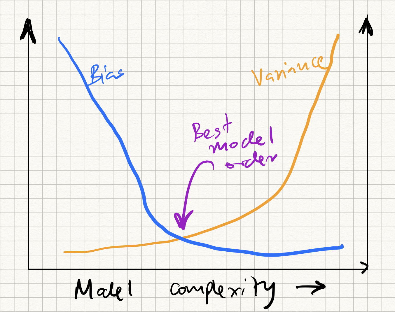
The question, then, is how to control the position on this curve so that we hit the sweet spot in the middle?

(It turns out that deep neural nets don’t quite obey this curve – a puzzling phenomenon called “double descent” occurs, but let us not dive too deep into it here; Google it if you are interested.)

We had previously introduced regularizers as a way to mitigate shortage of training samples, and in neural nets a broader class of regularization strategies exist. Simple techniques such as adding an extra regularizer do not work in isolation, and a few extra tricks are required. These include:

• Designing “bottlenecks” in network architecture: One way to regularize performance is to add a linear layer of neurons that is “narrower” than the layer preceding and succeeding it.

• Early stopping: We monitor our training and validation error curves during the learning process. We expect training error to (generally) decrease, and validation error to flatten out (or even start increasing). The gap between the two curves indicates generalization performance, and we stop training when this gap is minimized. The problem with this approach is that if we train using stochastic methods (such as SGD) the error curves can fluctuate quite a bit and early stopping may lead to sub-optimal results.

• Weight decay: This involves adding an L2-regularizer to the standard neural net training loss.

• Dataset augmentation: To resolve the imbalance between the number of model parameters and the number of training examples, we can try to increase dataset size. One way to simulate an increased dataset size is by artificially transforming an input training sample (e.g. if we are dealing with images, we can shift, rotate, flip, crop, shear, or distort the training image example) before using it to update the model weights. There are smarter ways of doing dataset augmentation depending on the application, and libraries such as PyTorch have inbuilt routines for doing this.

• Dropout: A different way to solve the above imbalance is to simulate a smaller model. This can be (heuristically) achieved via a technique called dropout. The idea is that at the start of each iteration, we introduce stochastic binary variables called masks – $m_i$ – for each neuron. These random variables are 1 with probability $p$ and 0 with probability $1-p$. Then, in the forward pass, we “drop” individual neurons by masking their activations:

\[h_i = m_i \phi(z_i)\]

and in the backward pass, we similarly mask the corresponding gradients with $m_i$:

\[\partial_{z_i} \mathcal{L} = \partial_{h_i} \mathcal{L} \cdot m_i \cdot \partial_{z_i} \phi (z_i) .\]

During test time, all weights are scaled with $p$ in order to match expected values.

• Transfer learning: Yet another way to resolve the issue of small training datasets is to transfer knowledge from a different learning problem. For example, suppose we are given the task of learning a classifier for medical images (say, CT or X-Ray). Medical images are expensive to obtain, and training very deep neural networks on realistic dataset sizes may be infeasible. However, we could first learn a different neural network for a different task (say, standard object recognition) and finetune this network with the given available medical image data. The high level idea is that there may be common learned features across datasets, and we may not depend on re-learning all of them for each new task.