Lecture 4: ConvNets

In which we introduce convnets and describe their many benefits.

Convolutional Neural Networks

Beyond fully connected networks

Thus far, we have introduced neural networks in a fairly generic manner (layers of neurons, with learnable weights and biases, concatenated in a feed-forward manner). We have also seen how such networks can serve very powerful representations, and can be used to solve problems such as image classification.

The picture we have for our network looks something like this:

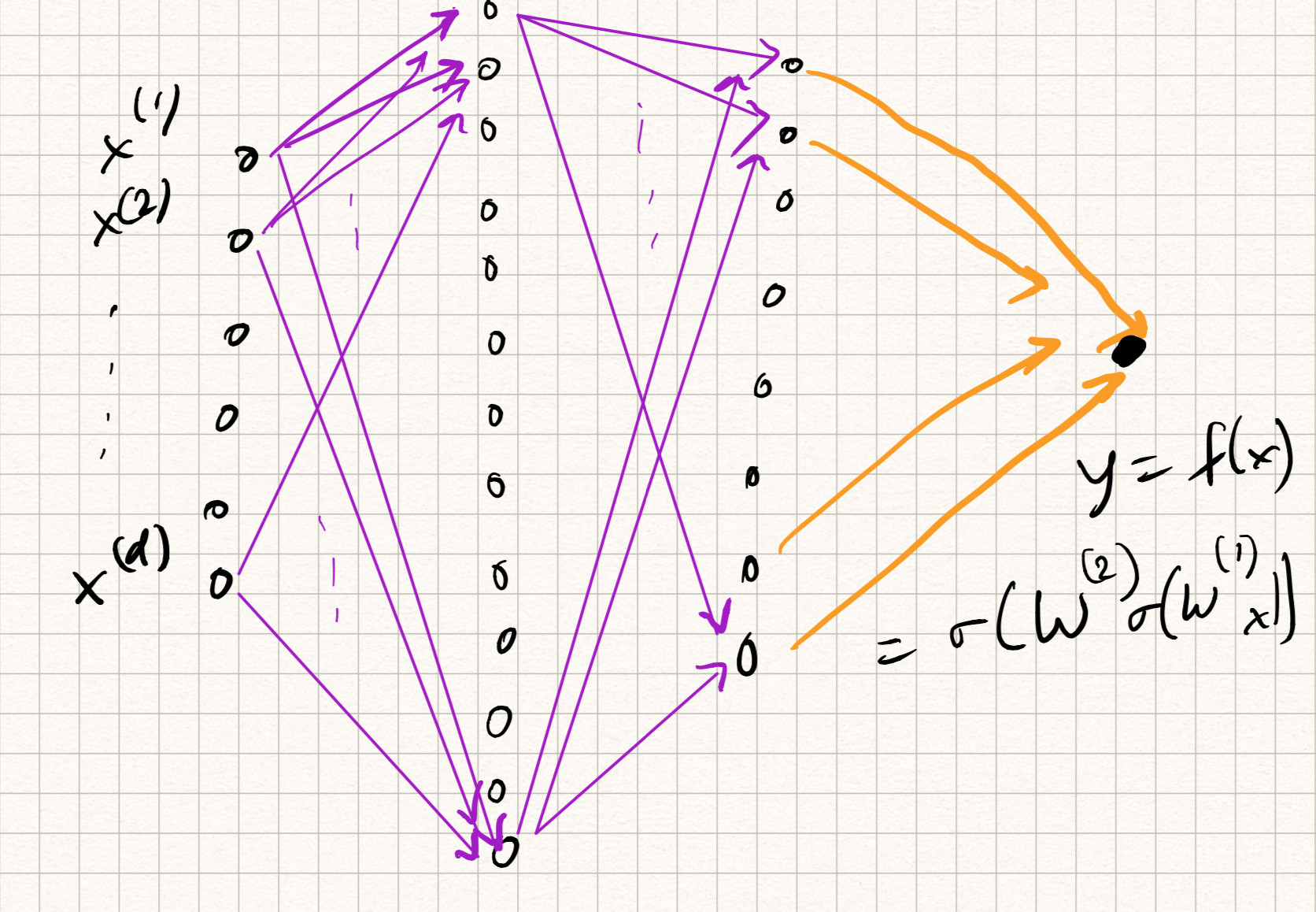
There are a few issues with this picture, however.

The first issue is computational cost. Let us assume a simple two layer architecture which takes a 400x400 pixel RGB image as input, has 1000 hidden neurons, and does 10-class classification. The number of trainable parameters is nearly 500 million. (Imagine now doing this calculation for very deep networks.) For most reasonable architectures, the number of parameters in the network roughly scales as $O(\tilde{d}^2 L)$, where $\tilde{d}$ is the maximum width of the network and $L$ is the number of layers. The quadratic scaling poses a major computational bottleneck.

This also poses a major sample complexity bottleneck – more parameters (typically) mean that we need a larger training dataset. But until about a decade ago, datasets with hundreds of millions (or billions) of training samples simply weren’t available for any application.

The second issue is loss of context. In applications such as image classification, the input features are spatial pixel intensities. But what if the image shifts a little? The classifier should still perform well (after all, the content of the image didn’t change). But fully connected neural networks don’t quite handle this well – recall that we simply flattened the image into a vector before feeding as input, so spatial information was lost.

A similar issue occurs in applications such as audio/speech, or NLP. Vectorizing the input leads to loss of temporal correlations, and general fully connected nets don’t have a mechanism to capture temporal concepts.

The third issue is confounding features. Most of our toy examples thus far have been on carefully curated image datasets (such as MNIST, or FashionMNIST) with exactly one object per image. But the real world is full of unpredictable phenomena (there could be occlusions, or background clutter, or strange illuminations). We simply will not have enough training data to robustify our network to all such variations.

Convolutional neural networks (CNNs)

Fortunately, we can resolve some of the above issues by being a bit more careful with the design of the network architecture. We focus on object detection in image data for now (although the ideas also apply to other domains, such as audio). The two Guiding Principles are as follows:

• Locality: neural net classifiers should look at local regions in an image, without too much regard to what is happening elsewhere.

• Shift invariance: neural net classifiers should have similar responses to the same object no matter where it appears in the image.

Both of these can be realized by defining a new type of neural net architecture, which is composed of convolution layers. Using this approach, we will see how to build our first truly deep networks.

Definition

A quick recap of convolution from signal processing. We have two signals (for our purposes, everything is in discrete-time, so they can be thought of as arrays) $x[t]$ and $w[t]$. Here, $x$ will be called the input and $w$ will be called the filter or kernel (not to be confused with kernel methods). The convolution of $x$ and $w$, denoted by the operation $\star$, is defined as:

\[(x \star w)[t] = \sum_\tau x[t - \tau] w[\tau] .\]

It is not too hard to prove that the summation indices can be reversed but the operation remains the same:

\[(x \star w)[t] = \sum_\tau x[\tau] w[t - \tau] .\]

In the first sense, we can think of the output of the convolution operation as “translate-and-scale”, i.e., shifting various copies of $x$ by different amounts $\tau$, scaling by $w[\tau]$ and summing up. In the second sense, we can think of it as “flip-and-dot”, i.e., flipping $w$ about the $t=0$ axis, shifting by $t$ and taking the dot product with respect to $x$.

This definition extends to 2D images, except with two (spatial) indices:

\[(x \star w)[s,t] = \sum_\sigma \sum_\tau x[s - \sigma, t - \tau] w[\sigma, \tau]\]

Convolution has lots of nice properties (one can prove that convolution is linear, associative, and commutative). But the main property of convolution we will leverage is that it is equivariant with respect to shifts: if the input $x$ is shifted by some amount in space/time, then the output $x \star w$ is shifted by the same amount. This addresses Principle 2 above.

Moreover, we can also address Principle 1: if we limit the support (or the number of nonzero entries) of $w$, then this has the effect that the outputs only depend on local spatial (or temporal) behaviors in $x$!

[Aside: The use of convolution in signal/image processing is not new: convolutions are used to implement things like low-pass filters (which smooth the input) or high-pass filters (which sharpen the input). Composing a high-pass filter with a step-nonlinearity, for example, gives a way to locate sharp regions such as edges in an image. The innovation here is that the filters are treated as learnable from data].

Convolution layers

We can use the above properties to define convolution layers. Somewhat confusingly, the “flip” in “flip-and-dot” is ignored; we don’t flip the filter and hence use a $+$ instead of a $-$ in the indices:

\[z[s,t] = (x \star w)[s,t] = \sum_{\sigma = -\Delta}^{\Delta} \sum_{\tau = -\Delta}^{\Delta} x[s + \sigma,t + \tau] w[\sigma,\tau].\]

So, basically like the definition convolution in signal processing but with slightly different notation – so this is only a cosmetic change. The support of $w$ ranges from $-\Delta$ to $-\Delta$. This induces a corresponding region in the domain of $x$ that influences the outputs, which is called the receptive field. We can also choose to apply a nonlinearity $\phi$ to each output:

\[h[s,t] = \phi(z[s,t]).\]

The corresponding transformation is called feature map. The new picture we have for our convolution layer looks something like this:

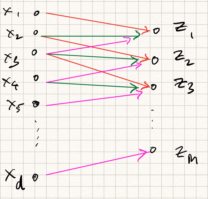
Observe that this operation can be implemented by matrix multiplication with a set of weights followed by a nonlinear activation function, similar to regular neural networks – except that there are two differences:

• Instead of being fully connected, each output coefficient is only dependent on $(2\Delta+1 \times 2\Delta+1)$-subset of input values; therefore, the layer is sparsely connected.

• Because of the shift invariance property, the weights of different output neurons are the same (notice that in the summation, the indices in $w$ are independent of $s,t$). Therefore, the weights are shared.

The above definition computed a single feature map on a 2D input. However, similar to defining multiple hidden neurons, we can extend this to multiple feature maps operating on multiple input channels (the input channels can be, for example, RGB channels of an image, or the output features of other convolution layers). So in general, if we have $D$ input channels and $F$ output feature maps, we can define:

\[\begin{aligned} z_i &= \sum_j x_j \star w_{ij} \\ h_i &= \phi(z_i). \end{aligned}\]

Combining the above properties means that the number of free learnable parameters in this layer is merely $O(\Delta^2 \times D \times F)$. Note that the dimension of the input does not appear at all, and the quadratic dependence is merely on the filter size! So if we use a $5 \times 5$ filter with (say) 20 input feature maps and 10 output feature maps, the number of learnable weights is merely $5000$, which is several orders of magnitude lower than fully connected networks!

A couple of more practical considerations:

• Padding: if you have encountered discrete-time convolution before, you will know that we need to be careful at the boundaries, and that the sizes of the input/output may differ. This is taken care of by appropriate zero-padding at the boundaries.

• Strides: we can choose to subsample our output in case the sizes are too big. This can be done by merely retaining every alternate (or every third, or every fourth..) output index. This is called stride length. [The default is to compute all output values, which is called a stride length of 1.]

• Pooling: Another way to reduce output size is to aggregate output values within a small spatial or temporal region. Such an aggregation can be performed by computing the mean of outputs within a window (average pooling), or computing the maximum (max pooling). This also has the advantage that the outputs become robust to small shifts in the input.

So there you have it: all the ingredients of a convolutional network.

Training a CNN

Note that we haven’t talked about a separate algorithm for training a convnet. That is because we do not need to: the backpropagation algorithm discussed in the previous lecture works very well!

The computation graph for CNNs is a bit different for the same reasons that conv layers are different from regular (dense) layers:

• the connections are sparse and local, so one needs to do some careful book-keeping.
• Also, the weights are shared, so we need to be a bit more careful while deriving the backward pass rules.

Fortunately, backprop translates very easily to convolutional networks, but let’s not derive the updates in detail here.

Practical Deep Networks

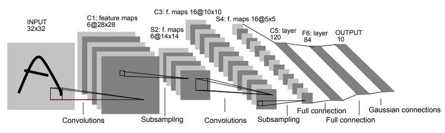
One of the first success stories of ConvNets was called LeNet, invented by LeCun-Bottou-Bengio-Haffner in 1998, which has the following architecture:

From 1998 to approximately 2015, most of the major advances in object detection were made using a series of successively deeper convolutional networks:

• AlexNet (2012), which arguably kickstarted the reemergence of deep neural nets in real-world applications. This resembled LeNet but with more feature maps and layers.

• VGGNet (2014), also similar but even bigger. The main innovation in VGG was the definition of a VGG block, a particular serial combination of convolutional + max-pool layers. The network itself was constructed by stacking together several such VGG blocks.

• GoogleNet (2014): this was an all-convolutional network (no fully connected layers anywhere, except the final classification).

• After 2015, deeper networks were constructed using residual blocks, which we will only briefly touch upon below.

Residual Networks

The origin of residual networks was somewhat accidental: in 2016, He and co-authors realized that instead of progressively modeling new features (by adding new convolutional layers), we could use the layers to model differences (or residuals). In some sense, each successive layer would predict “new information” that was not already previously extracted. So instead of the standard layer operation:

\[h_{l+1} = \sigma(W_l h_l)\]

where $W_l$ is either dense or convolutional, we could write a residual block as follows:

\[h_{l+1} = h_l + \sigma(W_l h_l)\]

and compose a residual network by composing several such blocks in serial.

In terms of the network, this action can be represented via a skip connection where there is a parallel path from the input $h_l$ to the output $h_{l+1}$ that bypasses the weights. [In practice, residual blocks are typically structured that the skip connections jumps over two layers of edges.]

This architectural difference sounds minor, but the effects are profound. In particular, the optimization landscape of residual networks is considerably easier than that of regular networks. Residual architectures are currently the core of all the best performing networks on image recognition benchmarks; see their details here.