Lecture 13: Self-supervised learning

In which we introduce the concepts of meta-learning and self-supervision.

Supervised (deep) learning has mainly gone after datasets such as MNIST or CIFAR-10/100, which have a small number of classes, and many samples per class.

But humans can generalize really well even with a very small number of examples per class! Think of the last time you saw the picture of an unknown animal. You clearly don’t need hundreds of examples in order to learn a concept.

Even worse: in several applications, you can’t get hundreds of examples anyway. Think of building an AI assistant to assist doctors in diagnosis: every test example may be new, critical cases are correlated with how rare they are, and large datasets are hard to find.

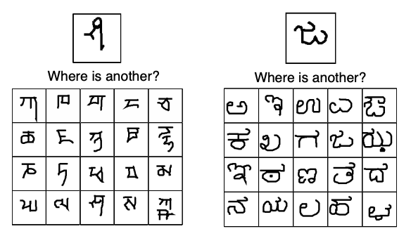
Therefore, it is of crucial importance moving forward to devise DL techniques that succeed with relatively few data points. An interesting early test bed is the Omniglot dataset, popularized in ML by Brendan Lake at NYU CDS, which can be thought of as “Transpose-MNIST” – lots of classes and very few samples per class. How do we effectively learn in this type of scenario?

Such problems fall into the realm of “few-shot” learning where “shots” here refer to the number of examples. For example, an n-class k-shot classification task requires learning to classify between $n$-classes using only $k$ (potentially $\ll n$) examples per class.

If an ML agent were given a $k$-shot dataset, how should it solve such a challenging task? The rapidly growing field of meta-learning advocates the following principles:

• each learning agent trying to solve a new task is guided by a higher-level meta-learner
• the meta-learner possesses meta-knowledge (in the form of features, or pre-trained nets, or other quantities) which is imparted to the learning agents when they are being trained.
• (here is the crux) the meta-learner itself can be trainable, and is able to learn from experience as it teaches different agents.

Transfer learning

Let us be concrete. A canonical example of the above approach iss transfer learning. We have actually already discussed transfer learning before (and implemented it for the case of R-CNN type object detection).

The high level idea is that given an ML task with a limited-sample dataset, one starts with a pre-trained base network that has already been trained on perhaps a bigger dataset (like ImageNet for images, or Wikipedia for NLP), and uses the given dataset to fine-tune to any new given task.

The problem, of course, is that one requires a good enough base model to start with. In the examples seen so far, the base model has been pre-trained using a massive dataset. The essence of pre-training is to get “good enough” features which generalize well for the given task, and it is not entirely clear if such “good enough” features could be learned in the few-shot setting. Below we will address more principled ways of performing transfer learning in the few-shot setting.

Model-agnostic meta learning (MAML)

Back to transfer learning. A different way of thinking about the few-shot learning problem is to visualize the tasks as different points in the parameter space. In this scenario, transfer learning/fine-tuning can be viewed as a souped-up initialization procedure where we initialize the weights at some known, excellent point in the parameter space, and use the available few-shot data to move the weights to some point better suited to the task.

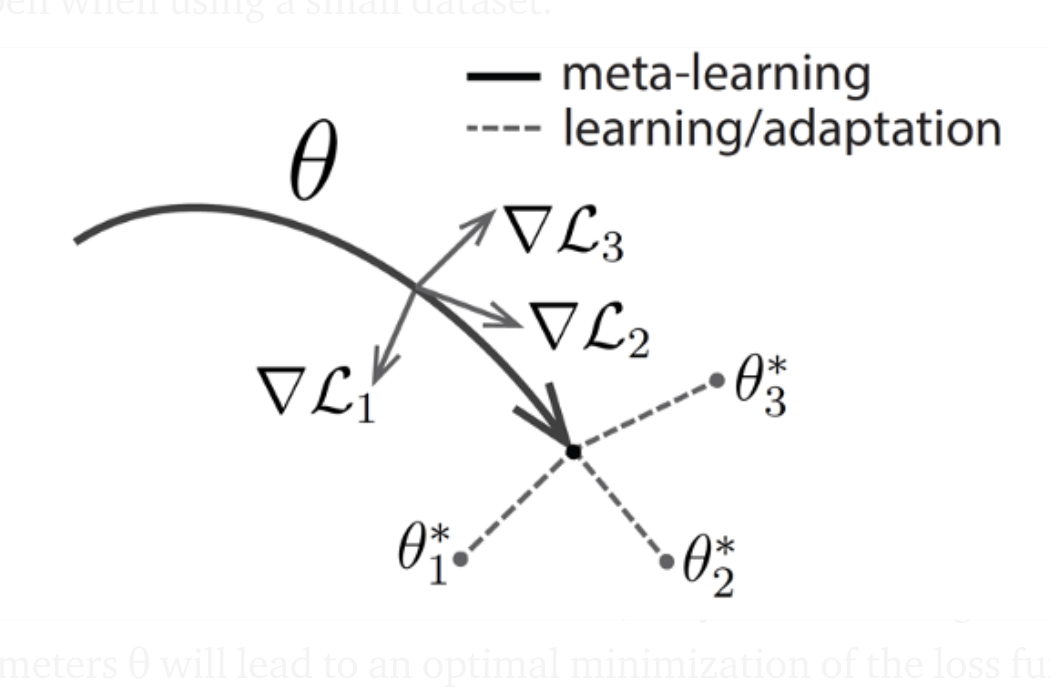
Of course, this assumes that the new task we are trying to learn is somehow close enough to the base model that it can be trained via a few steps of gradient descent. As different tasks are solved, can the meta-learner update the base model itself? If trained over sufficiently many tasks, then perhaps the base model is no longer required to be trained using a specific, large dataset – it can be a general model whose only goal is to be “fine-tunable” to different tasks using a few number of gradient descent steps. In that sense, this approach would be model-agnostic.

Let us formalize this idea (which is called model-agnostic meta-learning, or MAML). There is a base model $\phi$. There are $J$ different tasks. We use the base model $f_\phi$ – $\phi$ are the weights – as initialization. For each new task dataset $T_j$, we form a loss function (based on few-shot samples) $L(f_\phi, T_j)$ – this stands for the model $f$ with weights $\phi$ evaluated on training dataset $T_j$ – and fine-tune these weights using gradient descent. In the simplest case, if we used one step of gradient descent, this could be written as:

\[\phi_j \leftarrow \phi - \alpha \nabla_\phi L(f_\phi, T_j) .\]

If we used two steps of gradient descent, we would have to iterate the above equation twice. And so on. We use the final weights $\phi_j$ to solve task $T_j$.

The hope is that if the base model is good enough then the overall cumulative loss across different tasks at the adapted parameters is small as well. This is the meta-loss function:

\[M(\phi) = \sum_{j=1}^J L(f_{\phi_j},T_j) .\]

Notice the interesting nested structure:

• The meta-loss function $M(\phi)$ depends on the adapted weights $\phi_j$
• which in turn depend on the base weights $\phi$ via one or more steps of gradient descent.

So we can update the base weights themselves by summing up the gradients computed during the adaptation:

\[\begin{aligned} \phi &\leftarrow \phi - \beta \nabla_\phi M(\phi) \\ &= \phi - \beta \sum_j \nabla_\phi L(f_{\phi_j},T_j) \\ &= \phi - \beta \sum_j \nabla_\phi L(\phi - \alpha \nabla_\phi L(f_\phi, T_j)) . \end{aligned}\]

Some further observations:

• the “samples” in the above update correspond to different tasks. One could use stochastic methods here to speed things up: the meta-learner samples a new learning agents, “teaches” them how to update their weights by giving them the base model, and “learns” a new set of base model weights.
• “generalization” here corresponds to the fact that after a while, MAML learns parameters that can be adapted to new, unseen tasks via fine-tuning.
• the above equation is specific to the learning agents in MAML using one step of gradient descent. But one could use any other optimization method here – $k$-steps of gradient descent, SGD, Adam, Hessian methods, whatever – call this method $\text{Alg}$. Then a general form of MAML is:

\[\phi \leftarrow \phi - \beta \sum_j \nabla L(\text{Alg}_j)\]

The only requirement is that there is some way to take the derivative of $\text{Alg}$ in the chain rule – i.e., MAML works by taking the gradient of gradient descent!

One last point: The above gradient updates in MAML can be quite complicated. In particular, the meta-gradient update requires a gradient-of-a-gradient (due to the chain rule) and already needs tons of computations. If we want to increase this to $k$-steps of gradient descent, then we need higher-order gradients. A series of algorithmic improvements have improved this computational dependency on the complexity of the optimizer, but we won’t cover it here.

Metric embeddings

An alternative family of meta-learning approaches is learning metric embeddings. The high level idea is to learn embeddings (or latent representations) of all data points in a given dataset (similar to how we learned word embeddings in NLP). If the embeddings are meaningful, then the geometry of the embedding space should tell us class information (and we should be able to use simple geometric methods such as nearest neighbors or perceptrons to classify points).

An early approach (pioneered by LeCun and collaborators in the nineties and revived a few years ago) is Siamese Networks. The goal was to solve one-shot image classification tasks, where we are given a database of exactly one image in each class.

Imagine a training dataset $(x_1, x_2, \ldots, x_n)$. The label indices don’t matter here since all the points are of distinct classes. Siamese nets work as follows.

• set up a Siamese network (pair of identical, weight-tied feedforward convnets, followed by a second network). The first part (pair of identical networks) $f_\theta$ consists of a standard convnet mapping data points to some latent set of features; we use this to evaluate every pair of data points and get outputs $f_\theta(x_i)$ and $f_\theta(x_j)$.

• compute the coordinate-wise distances

\[g(x_i, x_j) = |f_\theta(x_i) - f_\theta(x_j) | .\]

This gives a vector which is a measure of similarity between the embeddings.

• Feed it through a second network that gives probabilities of matches, i.e., whether the two images are from the same class. A simple such network would :

\[p(x_i, x_j) = \sigma(W g(x_i, x_j))\]

• Apply standard data augmentation techniques (noise, distortion, etc) and train the network using SGD.
• Given a test image, match it with every point in the dataset. The final predicted class is the one with the max matching probability.

\[c(x) = \arg \max_{i \in S} P(x,x_i) .\]

This idea was refined to the $k$-shot case via Matching Networks by Vinyals and coauthors in 2016. The steps are similar to the ones above, except that we don’t compute distances in the middle, and use a trainable attention mechanism (instead of a standard MLP) to declare the final class:

\[c(x) = \arg \max_{i \in S} \sum_{i=1}^n \sum_{j = 1}^k a(x_{nk}, x) y_{nk} .\]

Other attempts along this line of work include:

• Triplet networks (where we use three identical networks and train with triples of samples $(x’, x’’, x^{-})$ – the first two from the same class and the last from a different class.
• Prototypical Networks
• Relation Networks

among several others.

Contrastive self-supervision

This idea of using Siamese networks to learn useful embedding features for unlabeled/few-shot datasets is rather similar to the next-sentence-prediction task that we used to learn BERT-style representations in NLP.

We can use similar techniques for other data types too! For example, imagine that we were trying to learn embeddings for image- or video- data. The Siamese network idea works here too – as long as we develop a contrastive pretext task that enables us to devise embeddings and compare pairs (or triples) of inputs. The above example of Siamese networks corresponded to a “same-class-classification” pretext task. But we could think of others:

• for images, one candidate pretext task could be to predict relative transformations: given two images, predict whether one is a rotation/crop/color transformation of the second, or not.

• for video, one candidate pretext task could be shuffle-and-learn where given three frames, the goal is to shuffle the order back to a temporally coherent manner.

• For audio-video, a candidate pretext task could be match whether the given audio corresponds to the video, or not.

• Jigsaw puzzles: the input is a bunch of shuffled tiles, and the goal is to predict a permutation.

All these methods have been applied to varying degrees of success, culminating in SIMCLR (by Hinton and co-authors) which reached AlexNet-level performance on image classification using 100X fewer labeled samples.

The idea in SimCLR is surprisingly simple: given an image $x$, a good model must be able to distinguish “positive” examples (e.g. all natural geometic transformations of this image, say $T(x)$), from “negative” ones (e.g. other images from a minibatch not related to this one.)

The way it implements this is via learning features by optimizing a contrastive loss. Given an image $x$, a positive example $x_+$ sampled from $T(x)$, and a set of negative examples $N$, SIMCLR does two things:

• Apply an encoder $g$ to all data points. Think of this encoder as (say) a standard ResNet.

• Apply a small “projection head” $h$ to map the encoder features to a space where the loss can be applied. This can be, for example, a shallow MLP similar to what we used for Siamese networks above.

• Let $z = h(g(x)), z_+ = h(g(x_+)), z_n = h(g(x_n))$. Take a gradient step that optimizes a cross-entropy style contrastive loss; here, $\tau$ is a learnable temperature parameter and $\sim$ is the cosine similarity between two vectors.

\[l = - \log \frac{\exp\left(\text{sim}(z,z_+)/\tau\right)}{\sum_{n \in N \cup \{z_+\}} \exp\left(\text{sim}(z,z_n)/\tau\right)}\]

Why does this loss make sense? Intuitively, starting from a totally unlabeled dataset we are setting up a classification problem where there are as many “classes” as samples in a minibatch. Therefore, a good feature embedding $g$ should learn to sufficiently separate out the different “classes”, i.e., group features corresponding to the same root image together while the rest far apart. In this sense, SIMCLR can be viewed as a considerable simplification of the Siamese Net idea.

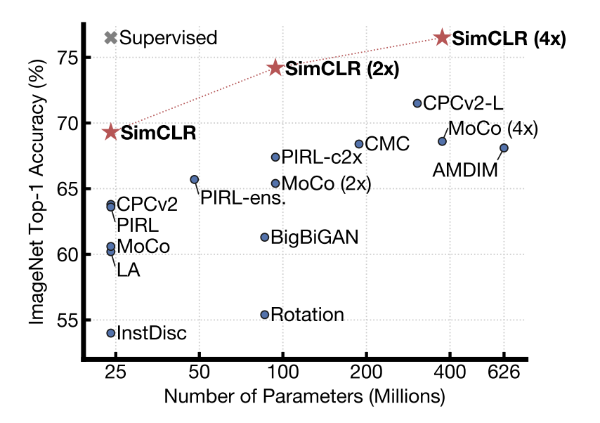
Once feature embeddings have been learned, we can drop the project head, and just use the feature encoder $g$. For any new downstream task (even with a small number of examples), we can then throw a linear classifier on top and either freeze the encoder weights/learn only the top layer, or fine-tune all the weights, depending on how much data is present. Here is a visualization of comparisons with other self-supervised baselines:

For a nice illustrated summary, see here.

Contrastive Language-Image Pretraining

Simple ideas that work (like SIMCLR) usually lead to good things. One (surprisingly powerful) offshoot is language-image feature learning.

Say we have a large, unstructured dataset of captioned images. This dataset can be acquired (say) by doing a search of FlickR or Instagram or something else.

Using this dataset, we can use a SIMCLR-style approach to learn a multi-modal feature encoder, having one tower of weights for the language part (call it $g_l()$), and one tower of weights (call it $g_v()$) for the image part. These weights should satisfy two properties:

• features learned by applying the image tower to an image, and the language to the corresponding caption, should be similar;
• image features should be far away from the caption of features of other images in the minibatch.

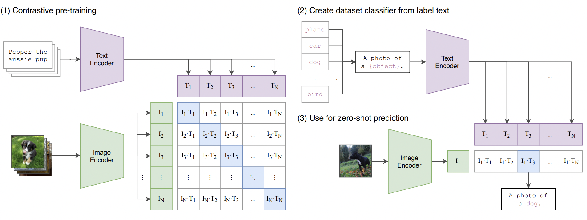
So, basically SIMCLR, except that the “transformation” backbone is removed, and replaced by one that processes a natural language caption! This approach is called CLIP (Contrastive Language-Image Pretraining), and this model serves as the feature extraction bedrock of more exciting, subsequent developments in unsupervised generative models (such as Dall-E 2 and Stable Diffusion). See the [CLIP paper] for details; this figure is a great illustration.

A few more CLIP-isms:

• Just as SIMCLR, we can do transfer learning by taking the image feature tower, throwing a linear layer on top, and finetuning to a new (given, small-size) dataset.

• A beautiful benefit of CLIP is the ability to do zero-shot transfer. Say we wanted to build an animal classifier, but our training dataset had zero images of (say) a woolly mammoth. This would be an entirely new class label (outside the set of known concepts), and in the standard supervised setup, there would be no way of recognizing this new concept.

  However, CLIP circumvents this as follows. To recognize the woolly mammoth, all we would have to provide is a caption in natural language describing the picture of a mammoth, something like “a photo of an animal that looks like an elephant but has brown fur and big tusks”.

  Why would this work? Notice that we not only learned good image features via CLIP; we also aligned the features with text descriptions. Therefore, generalization to new, totally unseen categories can effectively happen, if somehow we were able to map the new category to a string of already-seen language tokens.

  Technically speaking, this is not a fully unsupervised approach (there is the issue of coming with a suitable caption, or prompt), so this method can be viewed as weak language supervision.

Generative Pre-Training

Under construction.