Lecture 11: Generative Adversarial Networks

In which we introduce the concept of generative models and two common instances encountered in deep learning.

Much of what we have discussed in the first part of this course has been in the context of making deterministic, point predictions: given image, predict cat vs dog; given sequence of words, predict next word; given image, locate all balloons; given a piece of music, classify it; etc. By now you should be quite clear (and confident) in your ability to solve such tasks using deep learning (given, of course, the usual caveats on dataset size, quality, loss function, etc etc).

All of the above tasks have a well defined answer to whatever question we are asking, and deep networks trained with suitable supervision can find them. But modern deep networks can be used for several other interesting tasks that conceivably fall into the purview of “artificial intelligence”. For example, think about the following tasks (that humans can do quite well), that do not cleanly fit into the supervised learning:

• find underlying laws/characteristics that are salient in a given corpus of data.

• given a topic/keyword (say “water lily”), draw/synthesize a new painting (or 250 paintings, all different) based on the keyword.

• given a photograph of a face (with the left half blacked out), mentally visualize how the rest would look like.

• be able to quickly adapt to new tasks.

• be able to memorize and recall objects.

• be able to plan ahead in the face of uncertain and changing environments;

among many others.

In the latter part of the course we will focus on solving such tasks. Somewhat fortunately, the main ingredients of deep learning (feedforward/recurrent architectures, gradient descent/backpropagation, data representations) will remain the same – but we will put them together into novel formulations.

GANs

We will now discuss families of generative models that are able to accurately reproduce very “realistic” data, even in high dimensions (such as high resolution face images).

Certain tasks in ML have well defined objective functions. (For example, classification; the obvious metric here is the 0/1 loss, and cross-entropy is its natural continuous relaxation.)

Certain tasks don’t have a well-defined objective function. For example, if we ask a neural net to “draw a painting”, the loss function is not well-defined.

However, we can provide examples of paintings and hope to reproduce more of those. Mathematically, if there is a sub-manifold of all image data that correspond to paintings, we can think of it as a distribution, learn its parameters, and then sample from it. (This is roughly the philosophy we used last time, but note that we are not necessarily assigning likelihoods here.)

Let us use a different approach this time, and work backwards. Let’s say our generative model (which is a neural network) was able to generate a sample painting. Let’s say an oracle (or human) is available, who can eyeball the painting and returns YES if the sample painting is realistic enough, and NO if not. This piece of information can be viewed as a rough error signal — and if there was some way to “backpropagate” this error, we can use gradient descent to iteratively adjust the parameters of the network, and generate more and more samples until the sample output always passes the eye test.

Sounds like a good idea, except, having an actual human to check each sample is not feasible.

To resolve this issue, let us now assume that the oracle with a second neural network. We call this the discriminator or the critic, which — in principle — should be able to tell the difference between “real” data samples, obtained from nature, and “synthetic” data samples produced by the generator.

But this discriminator network itself needs to be trained in order to learn to distinguish between real and fake samples. The insight used in GANs is a clever bootstrapping technique, where the samples from the generator serve as the fake data samples and compared with a training dataset of real samples.

Moreover, the bootstrapping technique enables us to iteratively improve both the generator and the the discriminator. In the beginning, the discriminator does its job easily: the generator produces noise, and the discriminator quickly learns to figure out real vs fake. As training progresses, the generator begins to catch up, and the discriminator needs to adjust its parameters to keep up. In this way, GAN training can be viewed as a two-player game, where the goal of Player 1 (the generator) is to fool the discriminator, and the goal of Player 2 (the discriminator) is to not be fooled by the discriminator. This is called adversarial training, and hence the name “GAN”.

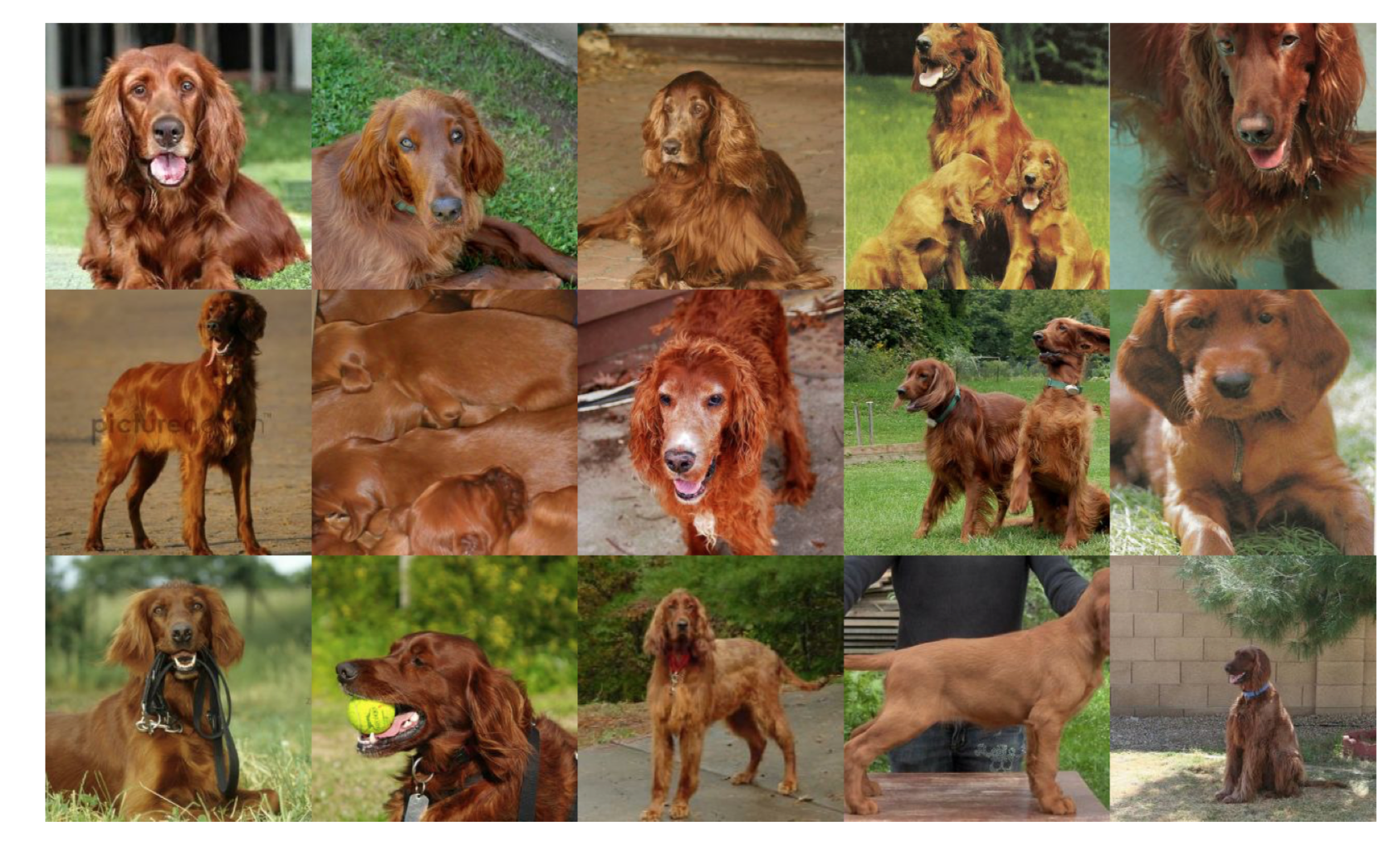
Somewhat interestingly, this type of learning procedure seems to achieve state-of-the-art generative modeling results. The results are impressive: can you figure out which of these dog images are fake and which are real?

Mathematics of GANS

Let us now cast the above discussion into a typical 3-step ML framework (representations, objective function, and optimization algorithm.)

We denote $G_\Theta(\cdot)$ to be the generator. Here, $\Theta$ represents all the weights/biases of the generator network. As mentioned above, unlike regular neural networks used for classification/regression, the network is architecture is “reversed” – it takes in as input a low-dimensional latent code vector $z$, and produces a high dimensional data vector (such as an image) as output. Recall that in a regular network, dimensionality is successively reduced through the layers (via pooling/striding); in a GAN generative network, dimensionality is successively expanded via upsampling or dilated/transpose convolutions.

We denote $D_\Psi(\cdot)$ to be the discriminator. This is a regular feedforward or convnet architecture, and produces an output probability of an input data sample being real or fake.

Let $y$ be the label where $y=1$ denotes real data and $y=0$ denotes fake data. For a given input, we will train the discriminator to minimize the cross-entropy loss:

\[L(\Psi) = - y \log D_\Psi(x) - (1-y) \log (1 - D_\Psi(x))\]

The first term disappears if $x$ is fake ($y=0$), and the second term disappears if $x$ is real ($y=1$). Fake data samples can be produced by sampling $z \sim \text{Normal}(0,I)$ and passing it through the generator network to produce $G_\Theta(z)$. So the loss function now becomes:

\[L(\Theta,\Psi) = - E_{x \sim \text{real}} \log D_\Psi(x) - E_{z \sim \text{Normal}(0,I)} \log (1 - D_\Psi(G_\Theta(z))) ,\]

where now the goal of the generator is to fool the discriminator as much as possible (i.e., maximize $L$). So the two-player game now becomes:

\[\max_\Theta \min_\Psi L(\Theta,\Psi) .\]

In the literature, it is conventional to flip min- and max-, and negate the loss function. So the standard GAN objective now becomes:

\[L(\Theta,\Psi) = E_{x \sim \text{real}} \log D_\Psi(x) + E_{z \sim \text{Normal}(0,I)} \log (1 - D_\Psi(G_\Theta(z)))\]

We now discuss how to train this network. In each iteration, we sample two minibatch of real data samples and fake data samples. Then, we form the above objective function and take gradients. The gradient with respect to the discriminator is used to update the weights $\Psi$ (note that since we are minimizing with respect to $\Theta$ and maximizing with respect to $\Psi$, this is an algorithm called gradient descent-ascent):

\[\begin{aligned} \Theta &\leftarrow \Theta - \eta \nabla_\Theta L(\Theta,\Psi) \\ \Psi &\leftarrow \Psi + \eta \nabla_\Psi L(\Theta,\Psi) \end{aligned}\]

In practice, other updates (such as Adam) may be used.

Note that due to all the hacks above, we cannot quite calculate likelihoods the way we do in the case of flow-models. For this reason, GANs are instances of likelihood-free generative models.

Challenges, extensions, and examples

There are a couple of issues with GAN training that we need to keep in mind.

One issue is the form of the loss itself. Observe above that the generator weights only get updated by the gradients of the second term:

\[\log (1 - D_\Psi(G_\Theta(z)))\]

since they do not appear in the first. The problem with this is that if the generator sample is really bad (as is typically the case in the beginning of training), then the discriminator’s prediction is close to zero, and since $\log (1- D)$ is very flat when $D \approx 0$ there is not enough ‘signal’ to move the generator weights meaningfully. Increasing learning rates do not seem to help. This is called the saturation problem in GANs.

To fix this, while updating generator weights, it is common to heuristically replace the second term in the GAN loss with:

\[- \log D_\Psi(G_\Theta(z))\]

A comparison of the two losses are shown below. This solves the saturation problem, but note that now the gradients close to zero are suddenly very high and training becomes unstable. Stably training GANs was a challenge faced by the community for quite some time (and continues to be a challenge), and a common resolution is to use Wasserstein GANs. We won’t get into the details here, but the high level idea is that the above GAN loss function can be viewed as a specific form of distance between probability distributions (called the Jensen-Shannon divergence), and this can be generated to other distances. A common alternative is the Earth-mover or Wasserstein distance, leading to a different type of GAN model called Wasserstein GAN. There is a lengthy derivation involved, but the loss function becomes:

\[L^{WGAN}_(\Theta,\Psi) = E_{x \sim \text{real}} f(D_\Psi(x)) + E_{z \sim \text{Normal}(0,I)} - f(D_\Psi(G_\Theta(z))) .\]

where $f$ is a monotonic function that is 1-Lipschitz. In practice, this property can be implemented via a procedure called gradient-clipping, but let’s not get into the weeds.

A third issue is something called mode collapse. If we stare closely, suppose that the network $G_\Theta(z)$ is accidentally trained such that it always produces a fixed output $\hat{x}$ no matter what the $z$ is (i.e., the range of $G$ collapses to a single point), and that the output $\hat{x}$ exactly matches a sample from the real dataset. This leads to zero loss, and hence is an optimal solution! So in some sense, the network has memorized exactly one data sample from the training dataset – so it has not really learned the distribution – but the GAN loss function does not really distinguish between the two regimes.

This is actually not an isolated occurrence. Even if the generator does not memorize a given data point, it could just memorize a set of weights to produce fake data points that somehow the discriminator does not do very well on. This is a consequence of the two-player game; the generator can “win” by finding a “cheat code” set of weights that is over-optimized to fool the particular discriminator, and not necessarily actually solving the game (of learning the probability distribution).

Mode collapse can be viewed as a specific form of overfitting, and there are a few ways to avoid this: early stopping helps; so does changing the objective function to encourage diversity in mini-batches; and so does adding noise to the discriminator/generator outputs (a la dropout).

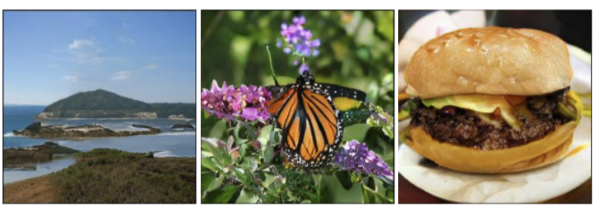
Lots more tricks to get GANs working (and we won’t get into all of them) here, but here are some representative images.

{ width=100% }

Conditional GANs

The above types of GAN models enable sampling from the data distribution: choose a random new latent code vector $z$ and generate a new sample $x = G(z)$.

In practice, however, it would be nice to have some kind of user control over the outputs. For example, the following applications:

• Category-dependent generation
• Image style transfer

Simple example: class-conditional GAN. Say MNIST digit. This is easy; we just augment the input $z$ with the class label $c$, and feed the same to the discriminator. So in some sense, a subset of features in the code vector fed to the generator are clearly interpretable as categorical input codes.

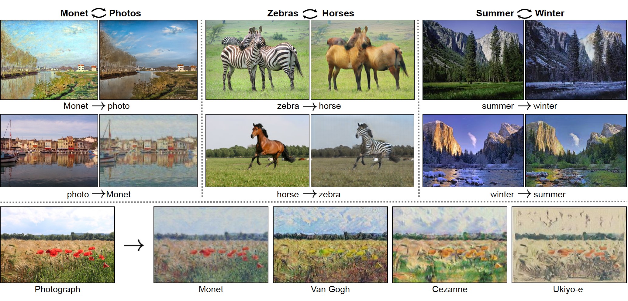
\[L(\Theta,\Psi) = E_{x \sim \text{real}} \log D_\Psi(x | c) + E_{z \sim \text{Normal}(0,I)} \log (1 - D_\Psi(G_\Theta(z | c)))\]

A harder problem is image style transfer. Say we want the content to remain the same but change the weather, or change night to day, or change artistic style. The issue with this kind of problem is that labels are hard to find (how do we get pairs of images with same content but different style?)

A way to achieve is this called cycle consistency. At a high level, the generative model consists of three networks simultaneously trained:

• Train two generative nets: $G_1$ for Style 1 to Style 2, and $G_2$ for style 2 back to Style 1.
• Use a discriminator to ensure that samples from $G_1$ (Style 2) are indistinguishable from real data.
• Use a reconstruction loss to make sure that $G_2$ learns to invert $G_1$.

Examples:

Variational Autoencoders

We won’t discuss VAEs in great detail. (The machinery is quite a bit involved, and they don’t work as well as GANs.) Autoencoders are fairly simple to understand. These consist of two networks $f_\theta$ and $g_\phi$, concatenated back-to-back trained using the reconstruction loss:

\[L(\theta,\phi) = \frac{1}{n} \sum_{i=1}^n \|x^{i} - f_\theta(g_\phi(x^{i})) \|^2 .\]

The simplest example of an autoencoder is when the functions $f_\theta$ and $g_\phi$ are single layers in a neural network with linear activation (i.e., linear mappings). Then the loss becomes:

\[L(U,V) = \frac{1}{n} \sum_{i=1}^n \|x^{i} - U V^T x^{i}) \|^2 .\]

which is equivalent to principal components analysis (PCA). The number of hidden units equals the number of principal components.

The output of $g_\phi$ can be viewed as a compressed representation of the input. This part is called the encoder, and the second part is called the decoder. Once this network is trained we can just take the decoder part and feed in different latent vectors to generate new samples, just like in GANs.

At a high level, variational autoencoders is an example of this approach. The architecture of a VAE looks like this:

where both the encoder and decoder represent probabilistic mappings. The loss function used to train this pair of network resembles the log-likelihood of the data samples (the same as that used to train normalizing flows/etc), but is augmented with a regularizer Kullback-Leibler Divergence, which encourages the distribution in the latent code ($z$-) space to become Gaussian; so the overall loss looks like this:

\[L_{\text{VAE}}(\theta,\phi) = - E_{z \sim q_\phi} \log p_\theta(x | z) + D_{KL}(q_\phi(z | x) || p_\theta(z))\]

which is minimized over both $\theta$ and $\phi$. We will skip the details; refer here for a rigorous treatment.