Lecture 11: Applications of Deep RL

In which we discuss success stories of deep RL, and the road ahead.

AlphaGo

A major landmark in deep learning research was the demonstration of AlphaGo in 2015, which was one of the success stories of deep RL in real(istic) applications.

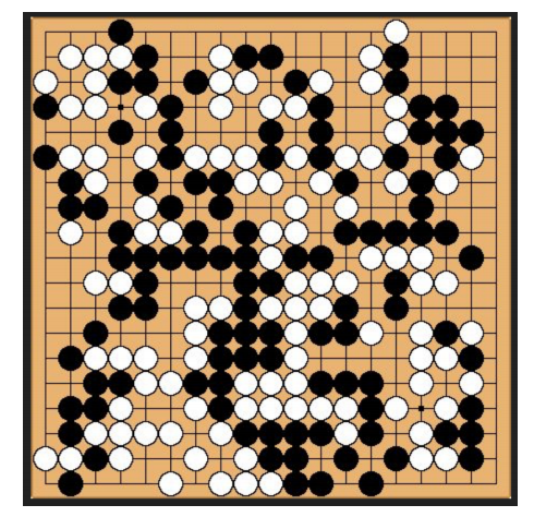
Go is a two-player board game where the players take turns placing black “stones” on a 19x19 grid, and the goal is to surround the opponents’ pieces and “capture” territory. The winner is declared by counting each player’s surrounded territory.

The classical way to solve such two player games (and other like Chess) via AI is to search a game tree, where each node in the tree is a game state (or snapshot) and children nodes are results of possible actions taken by each player. The leaves of the tree denote end states, and the goal of the AI is to discover paths to valuable/winning leaves while avoiding bad paths. Leaving aside the definition of “value”, this is obviously a very large tree in both Chess and Go with leaves the number of leaves being exponential in the depth (i.e., the number of moves in the game).

[An aside: in Chess after sufficiently many moves there is a particular phase called the Endgame, after which the winning sequence of moves are more or less well understood, and can be hard coded. Computer chess heavily relied on this particular trick; unfortunately, endgames in Go are way more complicated, and solving Go via computer was viewed as a major bottleneck.]

One way to reduce the number of possible paths is to perform Monte Carlo Tree Search, which was a crude form of estimating the Value function $V(s)$ of each state (i.e., each node in the tree) via random search.

The beauty of DeepMind’s AlphaGo (which was introduced in 2016) is that it completely eschews a tree-based data structure for representing the game. Instead, the state of the game is represented by a 19x19 black/white/gray image, which is fed into a deep neural network – just like how we would classify an MNIST grayscale image. The output of the network is the instantaneous policy, i.e., distribution over possible next moves. The architecture is a vanilla 13-layer convnet.

In fact, just this network is enough to do well in Go. One can train this in a standard supervised learning manner using an existing database of game-state/next-move pairs, and beat computer Go players based on tree search nearly 99% of the time! But top human players were able to beat this model.

But AlphaGo leverages the fact that we can do even better with RL. We can update the above network using self-play, where we create new games by sampling rollouts using the predicted distribution, measure rewards at the end of the game, and use the REINFORCE algorithm for further updating the weights.

In addition to the policy network trained above, AlphaGo also constructs a second network (called the value network) which, for a given state, predicts which player has advantage. In some sense, one can view this analogous to how we motivated GANs: the policy network proposes actions to take, and the value network evaluates how good different actions are in terms of expected return. [Such an approach is called an actor-critic method, which discuss below.] There were other additional hacks thrown on top to make everything work, but this is the gist. Read the (very enjoyable) paper if you would like to learn more.

Actor-critic methods

The high level idea in actor-critic methods is to combine elements from both policy gradients as well as Q-learning. Recall that the key idea in policy gradients was the computation of the update rule using the log-derivative trick:

\[\frac{\partial}{\partial \theta} \mathbb{E}_{\pi(\tau)} R(\tau) \approx R(s,a) \frac{\partial}{\partial \theta} \log \pi_\theta(a | s).\]

Here, for simplicity we have ignored trajectories and assumed that policies only depend on the current state of the world, and rewards only depend on the current action that we take. The policy network $\pi_\theta$ outputs a distribution over actions; favorable actions are associated with higher probabilities. We call this the actor network.

Instead of using the reward $R$ directly (which could be sparse, or non-informative), we instead replace this via the expected discounted reward, which is essentially the Q-function $Q(s,a)$. But where does this value come from? To compute this, we use a second auxiliary neural network (call it $Q_\phi$ where $\phi$ denotes this auxiliary network’s weights). We call this the critic network.

This sets up an interesting game theoretic interpretation. The actor learns to play the game, and picks the best moves at each time step. The critic learns to estimate values of different actions by the actor, and keeps track of long-term future rewards. There are other concepts involved here (such as advantage) and two time-scale learning which we won’t get into here; best left for a detailed course on RL.

The overall algorithm proceeds as follows:

1. Initialize $\theta, \phi, s$

2. At each time step:

   a. Sample $a’ \sim \pi_\theta(a’

   s_t)$

   b. Update actor network weights $\theta$ according to log-derivative trick

   c. Compute Bellman error $\delta_t$

   d. Update critic network weights $\phi$ according to Q-learning updates.

   e. Update state to $s_{t+1}$ and repeat!

AlphaFold2