Lecture 12: Diffusion Models

In which we discuss the foundations of generative neural network models.

Co-authored with Teal Witter.

Motivation

Much of what we have discussed in the first part of this course has been in the context of making deterministic, point predictions: given image, predict cat vs dog; given sequence of words, predict next word; given image, locate all balloons; given a piece of music, classify it; etc. By now you should be quite clear (and confident) in your ability to solve such tasks using deep learning (given, of course, the usual caveats on dataset size, quality, loss function, etc etc).

All of the above tasks have a well defined answer to whatever question we are asking, and deep networks trained with suitable supervision can find them. But modern deep networks can be used for several other interesting tasks that conceivably fall into the purview of “artificial intelligence”. For example, think about the following tasks (that humans can do quite well), that do not cleanly fit into the supervised learning:

• find underlying laws/characteristics that are salient in a given corpus of data.

• given a topic/keyword (say “water lily”), draw/synthesize a new painting (or 250 paintings, all different) based on the keyword.

• given a photograph of a face (with the left half blacked out), mentally hallucinate how the rest would look like.

• be able to quickly adapt to new tasks.

• be able to memorize and recall objects.

• be able to plan ahead in the face of uncertain and changing environments;

among many others.

In the next few lectures we will focus on solving such tasks. Somewhat fortunately, the main ingredients of deep learning (feedforward/recurrent architectures, gradient descent/backpropagation, data representations) will remain the same – but we will put them together into novel formulations.

Tasks such as classification/regression are inherently discriminative – the network learns to figure out the answer (or label) for a given input. Tasks such as synthesis are inherently generative – there is no one answer, and instead the network will need to figure out a probability distribution (or, loosely, a set) of possible answers to it. Let us see how to train neural nets that learn to produce such distributions.

[Side note: machine learning/statistics has long dealt with modeling uncertainty and producing distributions. Probabilistic models for machine learning is a vast area in itself (independent of whether we are studying neural nets or not). We won’t have time to go into all the details – take an advanced statistical learning course if you would like to learn more.]

Setup

Let us lay out the problem more precisely. In terms of symbols, instead of learning weights $W$ that learn a discriminative function mapping of the form: \(y = f_W(x)\) we will instead imagine that the space of all $x$ is endowed with some probability distribution $p(x)$. This may be a distribution that is without any conditions (e.g., all face images $x$ are assigned high values of $p(x)$, and the set of all images that are not faces are assigned low values of $p(x)$). Or, this may be a conditional distribution $p(x; c)$. (Example: the condition $c$ may denote hair color, and the set of all face images with that particular hair color $c$ will be assigned higher probability versus the rest).

If there was some computationally easy way to represent the distribution $p(x)$, we could do several things:

• we could sample from this distribution. This would give us the ability to synthesize new data points.

• we could evaluate the likelihood of a given test data point (e.g. answering the question: does this image resemble a face image?)

• we could solve optimization problems (e.g. among all potential designs of handbags, find the ones that meet color and cost criteria)

• perhaps learn conditional relationships between different features

etc.

The question now becomes: how do we computationally represent the distribution $p(x)$? Modeling distributions (particularly in high-dimensional feature spaces) is not easy – this is called the curse of dimensionality — and the typical approach to resolve this is to parameterize the distribution in some way: \(p(x) := p_\Theta(x)\) and try to figure out the optimal parameters $\Theta$ (where we will define what “optimal” means later).

Classical machine learning and statistical approaches start off with simple parameterizations (such as Gaussians). Gaussians are nice in many ways: they are exactly characterized by their mean and (co)variance. We can draw samples easily from Gaussians. Central limit theorem = any set of independent samples averaged over sufficiently many draws resembles a Gaussian. Computationally, we like Gaussians.

Unfortunately, nature is far from being Gaussian! Real-world data is diverse; multi-modal; discontinuous; involves rare events; and so on, none of which Gaussians can handle very well.

Second attempt: Gaussian mixture models. These are better (multi-modal) but still not rich enough to capture real datasets very well.

Enter neural networks. We will start with some simple distribution (say a standard Gaussian) and call it $p(z)$. We will generate random samples from $p$; call it $z$. We will then pass $z$ through a neural network: \(x = f_\Theta(z)\) parameterized by $\Theta$. Therefore, the random variable $x$ has a different distribution, say $p(x)$. By adjusting the weights we can (hopefully) deform $p(z)$ to obtain a $p(x)$ that matches any distribution we like. Here, $z$ is called the latent variable (or sometimes the code), and $f$ is called the generative model (or sometimes the decoder).

How are $p(x)$ and $p(z)$ linked? Let us for simplicity assume that $f$ is one-to-one and invertible, i.e., $z = f_\Theta^{-1}(x)$. Then, we can use the Change-of-Variables formula for probability distributions. In one dimension, this is fairly intuitive to understand: in order to conserve mass, the area of the intervals must be the same, i.e., $p(x)dx = p(z)d(z)$ and hence the probability distributions must obey:

\[p(x) = p(z) | \frac{dx}{dz} |^{-1}\]

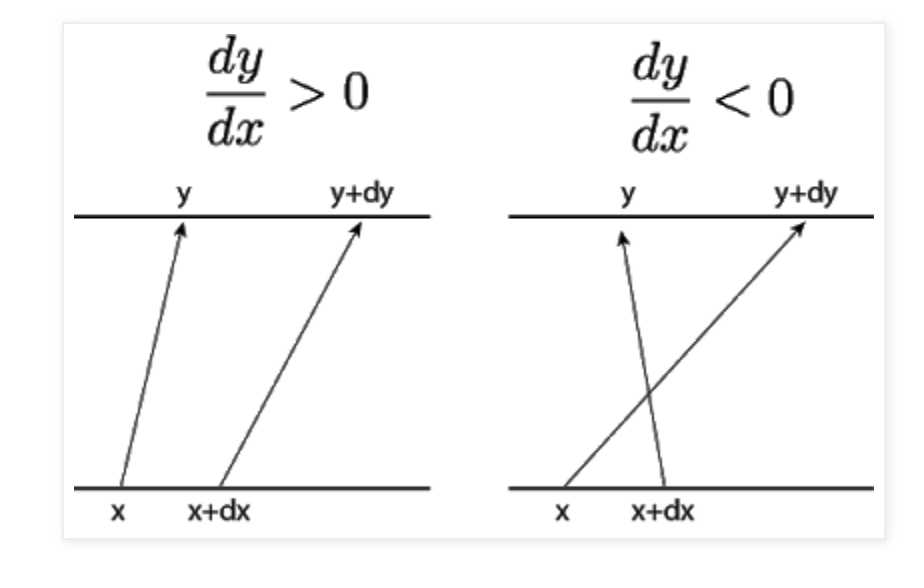
When both $x$ and $z$ have more than one dimension, we have to replace areas by (multi-dimensional) volumes and derivatives by partial derivatives. Fortunately, volumes correspond to determinants! Therefore, we can get an analogous formula by replacing the absolute value by the determinant of the Jacobian of the mapping $x = f(z)$:

\[p(x) = p(z) | \frac{\partial x}{\partial z} |^{-1}\]

This gives us a closed-form expression to evaluate any $p(x)$, given the forward mapping. However, note that for this formula to hold, the following conditions must be true:

• $f$ must be one-to-one and easily invertible.

• $f$ needs to be differentiable, i.e., the Jacobian must be well-defined.

• The determinant of the Jacobian must be easy to invert.

Reversible Models

As a warmup, a simple approach that ensures all of the above conditions are called reversible models. Recall the residual block that we discussed in the context of CNNs: this is similar. Residual blocks implement: \(x = z + F_\Theta(z)\) where $F_\Theta$ is some differentiable network that has equal input and output size. (You can use ReLUs too but strictly speaking we should use differentiable nonlinearities such as sigmoids). Typically, $F_\Theta$ is a dense shallow (single- or two-layer network).

Reversible models use the above block as follows. We will consider two auxiliary random variables $u$ and $v$ as the same size as $x$ and $z$, and define two paths: \(\begin{aligned} x &= z + F_\Theta(u), \\ v &= u . \end{aligned}\) The variable $u$ is called an additive coupling layer. If you don’t like adding an extra variable for memory reasons (say), you can just split your features into two halves and proceed.

The advantage of this model is that the inverse of this forward model is easy to calculate! Given any $x$ and $v$, the inverse of this model is given by: \(\begin{aligned} u &= v, \\ z &= x - F_\Theta(u) . \end{aligned}\)

What about the determinant of the Jacobian? Turns out that reversible blocks have very simple expressions for the determinant. For each layer, the Jacobian is of the form: \(\left( \begin{array}{cc} \frac{\partial x}{\partial z} & \frac{\partial x}{\partial u} \\ \frac{\partial v}{\partial z} & \frac{\partial v}{\partial u} \end{array} \right) = \left( \begin{array}{cc} I & \frac{\partial F_\theta}{\partial u} \\ 0 & I \end{array} \right)\) which is an upper-triangular matrix with diagonal equal to 1. Such matrices have determinant equal to 1 always (and such transformations are hence called “volume preserving”). In other words, each reversible block maps a set to another set of the same volume.

Having defined a single reversible block, we can now chain multiple such reversible blocks into a deeper architecture by alternating the roles of $x$ and $v$. Let’s say we have a second such block $F_\Psi$ applied to $v$ and $u$. Then, we get the following two-layer architecture: \(\begin{aligned} x' &= z + F_\Theta(u) \\ z' &= u + F_\Psi(x') \end{aligned}\)

(Exercise: can you compute the inverse of this two-layer block?)

Turns out that each such block is volume preserving, and hence the determinant of the overall Jacobian (no matter how many blocks we stack) are all equal to unity. We can think of each layer as incrementally changing the distribution until we arrive at the final result. Such a model that implements this type of incremental change is called a “flow” model. (The specific form above was called NICE – short for Nonlinear Independent Components Estimation).

We finally come to training this model. Different objective functions can be used: a common one is maximum likelihood: given a dataset of $n$ samples $x_1, x_2, \ldots, x_n$ we optimize for the parameters that maximize the overall likelihood: \(L(\Theta) = \prod_{i=1}^n p_X(x_i) = \prod_{i=1}^n p_Z(f^{-1}(x_i))\) where $p_Z$ is the base distribution. (Note that the Jacobian disappears.) In practice, sums are easier to optimize than products, and therefore we use the log-likelihood instead.

Normalizing Flows

Reversible blocks are nice from a compute standpoint, but have architectural limitations due to the volume preserving constraint.

Normalizing Flows (NF) generalize the above technique, and allow the mapping to be non-volume preseerving (NVP). The idea is to assume an arbitrary series of maps: $f_1, f_2, \ldots, f_L$ (where $L$ is the depth), so that: \(x = f_L \odot \ldots \odot f_2 \odot f_1(z) .\) Define $z_0 := z$ and $z_i$ as the output of the $i$-th layer. Applying the change-of-variables formula to any intermediate layer, we have the distributional relationship: \(\log p(z_i) = \log p(z_{i-1}) - \log | \text{det} \frac{\partial z_i}{\partial {z_{i-1}}} |.\) and recursing over $i$, we have the log likelihood: \(\log p(x) = \log p(z) - \sum_{i=1}^L \log | \text{det} \frac{\partial z_i}{\partial z_{i-1}} .\) This is a bit more complicated to evaluate, but in principle it can be done.

To make life simpler, in NF, we use the same principles as we did for reversible architectures:

• easy inverses for each layer

• easy Jacobian determinant

but this time, instead of creating an additive coupling layer $u$, we use an affine coupling layer: \(\begin{aligned} x &= z \odot \exp(F_\Theta(u)) + F_\Psi(u), \\ v &= u . \end{aligned}\) where $F_\theta$ and $F_\Psi$ are trainable functions, and $\odot$ is applied component wise. The inverse of the affine coupling layer is simple: \(\begin{aligned} u &= v, \\ z &= (x - F_\Psi(u)) \odot \exp(-F_\Theta(u)). \\ \end{aligned}\) Moreover, the Jacobian has the following structure: \(J = \left( \begin{array}{cc} \frac{\partial x}{\partial z} & \frac{\partial x}{\partial u} \\ \frac{\partial v}{\partial z} & \frac{\partial v}{\partial u} \end{array} \right) = \left( \begin{array}{cc} \text{diag}(\exp(F_\Theta(u))) & \frac{\partial F_\theta}{\partial u} \\ 0 & I \end{array} \right)\) which is an upper-triangular matrix, but with an easy-to-calculate determinant: \(det(J) = \exp(\sum_{i=1}^d F^{i}_\theta(u)).\)

Diffusion models

Motivation

We had previously discussed generative adversarial networks (GANs). GANs create realistic images by playing a game between two neural networks called the generator and discriminator; the generator learns to create realistic images while the discriminator learns to differentiate between these fake images and the real ones. Unfortunately, GANs suffer from a problem called mode collapse. During training, the generator can memorize a single image from the real data set and the discriminator (correctly) determines that the image is real. The problem is that training stops because the generator has achieved minimum loss. Now, we’re stuck with a generator that only outputs one image (to be fair, the one image does look real).

There have been several attempts to mitigate mode collapse by trying different loss functions (a loss function based on Wasserstein distance is particularly effective) and adding a regularization term (the idea is to force the generator to use the random noise it’s given as input). However, these and similar approaches cannot completely prevent mode collapse.

So we’re left with the same problem we had before: how to generate realistic images. Instead of GANs, the deep learning community has recently turned to diffusion …and the results are astounding. The basic idea of diffusion is to repeatedly apply a de-noising process to a random state until it resembles a realistic image. Let’s dive into the details.

Diffusion Process

Our goal is to turn random noise into a realistic image. The starting point of diffusion is the simple observation that, while it’s not obvious how to turn noise into a realistic image, we can turn a realistic image into noise. In particular, starting from a real image in our data set we can repeatedly apply noise (typically drawn from a normal distribution) until the image becomes completely unrecognizable. Suppose $x_0$ is the real image drawn from our data set. Let the first noised image be $x_1 = x_0 + \epsilon_1$ where the noise $\epsilon_1$ is drawn from a normal distribution $\mathcal{N}(\mathbf{0}, \sigma^2 \mathbf{I})$ for some variance $\sigma$. In this way, we can generate $x_{t} = x_{t-1} + \epsilon_{t}$ where $\epsilon_{t}$ is again drawn from the same distribution. We end up with a sequence $x_0, x_1, \ldots, x_T$ where the total number of steps $T$ is chosen so that $x_T$ looks entirely meaningless.

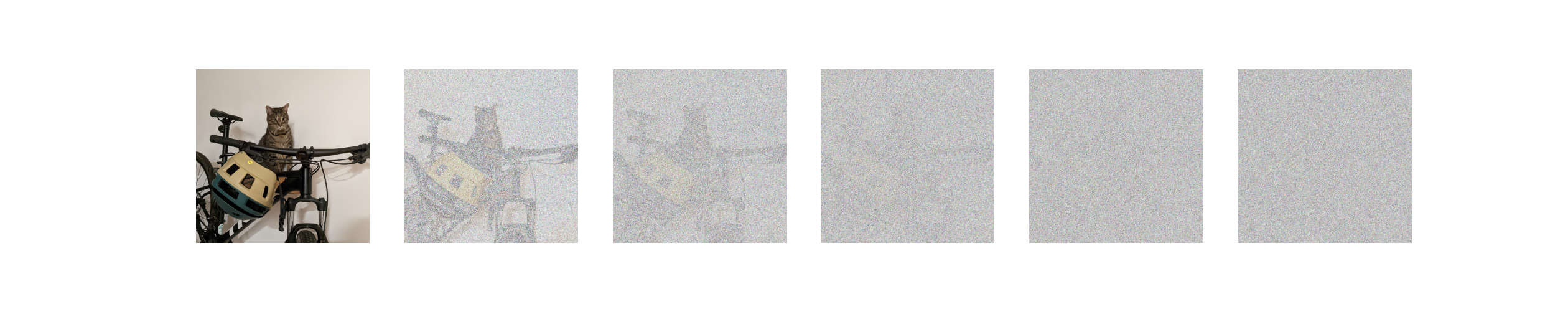
In this example, we turned a picture of Stripes on a bike into complete gibberish by adding normal noise five times. The key insight is that if we look at this sequence backwards then we have training data which we can use to teach a model how to remove noise.

Formally, the training data consists of $x_t$, $t$, and $x_{t-1}$. Our goal is to train a model $f_\theta$ to predict $x_{t-1}$ from $x_t$ and $t$. A very natural choice of loss function is then

\(\mathcal{L}(\theta) = \mathbb{E} [\| x_{t-1} - f_\theta(x_t, t) \|^2]\) where the expectation is over $x_t$, $t$, and $x_{t-1}$. However, researchers have found that it’s actually better for $f_\theta$ to predict the noise $\epsilon_{t}$ and then subtract it from $x_t$ to get $x_{t-1}$. Formally, the loss function is

\(\mathcal{L}(\theta) = \mathbb{E} [\| \epsilon_{t} - f_\theta(x_t, t) \|^2]\) where the expectation is again over $x_t$, $t$, and $x_{t-1}$ which induces $\epsilon_t = x_t - x_{t-1}$.

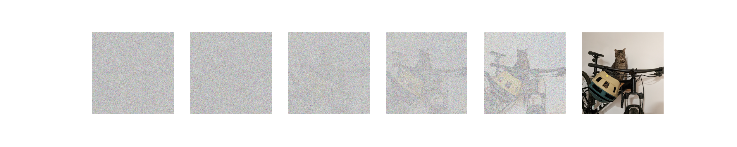
Once we have have a working $f_\theta$, we can use it to generate realistic images. We start with random noise which we’ll call $x_T’$. Then for $t=T,\ldots, 1$, we predict $\epsilon_t’ = f_\theta(x_t’, t)$ and compute $x_{t-1}’ = x_t’ - \epsilon_t’$. The final result $x_0’$ is what the diffusion process outputs. With any luck, this output is a realistic image.

Thinking back to our three-step recipe for machine learning, we have the loss function and optimizer (SGD, as usual) but how do we choose a good architecture?

Autoencoders and U-Nets

We’ll start with a high level description of autoencoders, work our way to u-nets, and then tie it all back to diffusion. I like to think about autoencoders in relation to GANs. Recall that GANs go small-big-small: they turn a small noise vector into an image (using the generator) and then convert the image into a scalar representing its realness (using the discriminator). In contrast, autoencoders go big-small-big: they compress a real image into a small embedding (using the encoder) and then reconstruct the original image from the embedding (using the decoder).

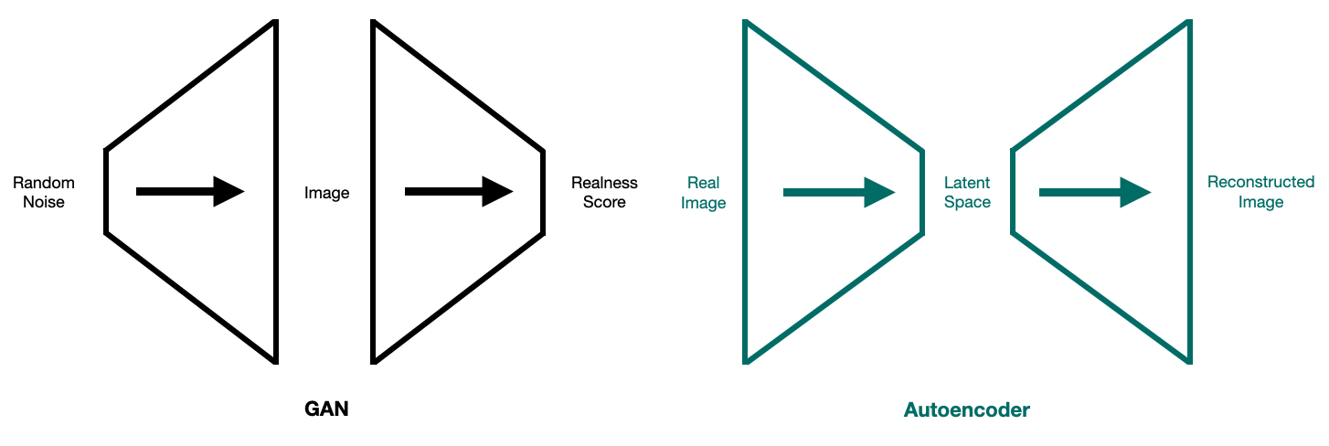
We can also think of the architecture of autoencoders in relation to GANs. Just like the discriminator, the encoder uses convolutional layers to go “small” while, just like the generator, the decoder uses tranposed convolutional layers to go “big”. The loss function typically used for autoencoders is the ($\ell_2$-norm) difference between the real image and the reconstructed image.

The real benefit of autoencoder architectures is that we get a meaningful representation of an image that somehow captures its “inherent” properties. In our current setting, one might think we can use this inherent meaning to differentiate the true content of the image from noise. And that’s exactly the motivation for the architecture we’ll use for the diffusion model.

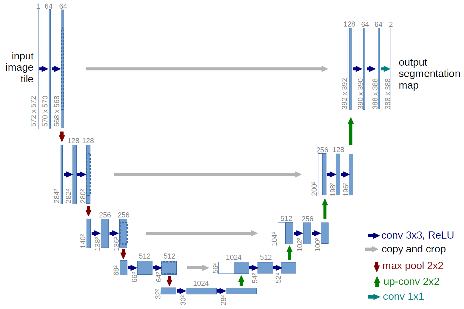
In particular, we’ll use what’s called a u-net. The u-net consists of convolutions and transposed convolutions tied together with pooling and residual connections. The model gets its distinctive name from the shape of its architecture (see below).

[[Source]](https://lmb.informatik.uni-freiburg.de/people/ronneber/u-net/)

Diffusion in Latent Space

At this point, we have the loss function, architecture, and optimizer for diffusion. What more could we need? Well, one nagging issue is that we’re adding and predicting noise in the high-dimensional pixel space (the space gets even larger if we want higher resolution!). This presents a computational problem since we’ll need lots of parameters and compute for our u-net. One novel contribution of stable diffusion is to apply the autoencoder idea again in a different way.

Looking at the first few noised versions of Stripes in our example, we could probably differentiate the noise (or at least identify his vague outline). But, to a computer, the visual properties of the pixel space that we’re so sensitive to are useless. We might as well embed the images into a latent space which captures more meaning. Then, within the latent space, we build a model to convert noise to an embedding of a realistic image. Once we have the final output of the diffusion process, we decode into an image that we can understand. This is exactly what stable diffusion does and, in as a result, it gains the efficiency of working in a smaller, more meaningful space.

Text Conditioning

The really cool part of stable diffusion is that it generates an image of any text prompt we give it. But we’ve only talked about diffusion as an unconditional process for turning noise into realistic images. What we want is a way of guiding the u-net through the denoising process so that it generates an image close to the text prompt we give it. We accomplish this by embedding the training images and their text descriptions in the same latent space. Using contrastive language image pretraining (CLIP), we ensure that the embedding of an image is close to the embedding of its description.

Now, we train the u-net on the embedded noised image $x_t$, the number of noise steps $t$, and the embedded text description $w$ of the original embedded image $x_0$. Formally, our goal is for $f_\theta(x_t, t, w) \approx \epsilon_t$. But how do we feed the u-net the embedded text in a meaningful way? Stable diffusion uses an architecture with cross-attention heads after the residual connection. The cross-attention is between the embedded text and the u-net’s representation of the embedded image. Intuitively, cross-attention gives the u-net a way of conditioning the de-noising process on the text description. This is very helpful: if we were told a noisy image depicts on a cat on a bike, we would see it differently than if we were told it depicts a flying turtle.

Once we have a working $f_\theta$, we can guide it through the denoising process with an embedded text prompt $w$. We start with noise in the latent space $x_T’$ and for $t=T, \ldots, 1$, we predict $\epsilon_t’ = f_\theta(x_t’, t, w)$ and compute $x’_{t-1} = x_t’ - \epsilon_t’$. Stable diffusion then decodes $x_0’$ into pixel space and, with any luck, the result is an image of the text prompt we started with.