Lecture 5: Object Detection

In which we explore applications of convnets in computer vision.

ConvNets in Computer Vision

Until now, we have discussed what convolutional networks are, and how they work. Now we will discuss where they are used.

While convnets are applicable in a wide variety of contexts, they are particularly relevant in the context of computer vision applications. This is because the two key properties of convnets – locality and shift invariance – are particularly relevant for natural image data.

Specifically, images naturally exhibit locality. For concreteness, imagine an image of an outdoors scene in a busy road. It is not hard to see that the raw image features (i.e., pixel intensities) are correlated spatially. Adjacent groups of pixels, depending on what scale you are interested in, convey information about edges/corners, or shapes (say squares/circles/etc), or object parts (say, a wheel), or objects themselves (say, cars/bikes/trucks/etc), or object contexts (say, a car on a road), all the way to the entire scene itself. The localized feature extraction capability of convnets, along with the ability for different layers to act at multiple scales (due to pooling), is perfect for extracting such information.

Secondly, images also exhibit (some degree of) shift invariance. This can be intuitively understood as follows: in the above example, if the camera position shifted a little bit, the contents of the captured image do not change by much (except maybe at the boundaries – which is why the choice of padding in convnets makes a difference!), but the raw features change quite dramatically (since all the pixel values get translated). So one would expect a good ML model to extract relevant information that is robust to such shifts, and convnets attempt to offer this by design.

(It is important to keep in mind that this is only a rough analogy. If we shift the position of the camera by more than a certain amount, we would expect even the contents of the image to dramatically change. There are other complications that arise due to finite camera resolutions, sensitivity of convnets to the pooling operation, and so on – so take this only as a guiding principle and not hard and fast rules.)

A perfect ML model for computer vision would also exhibit scale invariance as well as rotation invariance, since the contents of an image do not change by much if the camera pans/zooms/tilts by a small amount. A conv layer, as defined, does not provide scale invariance; however, convnets are usually constructed by stacking conv layers with pooling layers that successively group information from neighboring features, thus simulating multiple scales.

Object Detection

The most common application of convnets in computer vision is image classification, where the goal is to either declare whether an image present in an image or not. We have already seen enough examples of image classification (and indeed, classification is the canonical example given in most intro-ML courses) so we won’t dwell upon this too much further.

Object detection is a somewhat more challenging problem than classification. The goal here is to answer both “what is in the image?” and “where is it located?”

Let us frame the “where” question mathematically. One way to approach this problem is via model explanations. Assuming that an image has been classified using a regular convnet. One can ask: “which pixels (or features) in the image contributed the most to a particular classification result?” Notice there that there is no additional supervision assumed here; all we are given is a particular deep model acting on a particular test image, and we are asked to explain why it produced a particular answer.

This line of thinking is part of a bigger sub-area in deep learning called “interpretable learning”. There is a whole host of techniques within this area, some of which include:

• CAM (class activation mapping),
• gradient-based CAM, or GradCAM,
• LIME (linear interpretable model-agnostic explanations)

among many others. They all have their pros and cons, but here is a a quick explanation of GradCAM.

Suppose the class label of a particular test image is declared as $c$. Imagine the feature maps provided by any convolution layer, $A^k_{ij}$ (here, $i,j$ indicate spatial indices, and $k$ the channel index), and let $y^c$ be the pre-softmax output from the dense layer. Then, we compute the “neuron importance weight”:

\[\alpha_k^c = \frac{1}{Z} \sum_i \sum_j \frac{\partial y^c}{\partial A^k_{ij}}\]

This can be interpreted as a sensitivity score and tells us how much a unit change in the feature activations of a particular feature map would contribute to a particular class activation, marginalized over all the spatial indices. Next, we compute a heatmap:

\[L^c_{ij} = ReLU\left( \sum_k \alpha_k^c A^k_{ij} \right) .\]

which we calculate for every $i,j$. The ReLU is used to only indicate positive influence of the features on the class of interest. Here are some representative results, taken from the GradCAM paper:

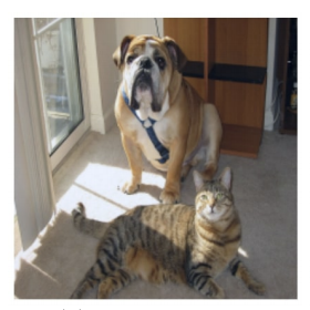
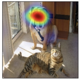
So we see that the results align well with human intuition: the “cat” class produces a heatmap that is correlated with cat features, while the “dog” class produces a heatmap that is correlated with dog features.

Unfortunately none of the above methods work on general data; even in the above (cherry-picked) examples we can start arguing with whether the heatmap really did capture all the relevant features corresponding to the correct class, or not. The jury is out as to what “interpretable deep learning” really means, and how that would look like.

Object Detection

Deep object detectors do not merely return a yes/no (or a one-hot vector encoding the class), but also a bounding box asking where in the image the object is present. The fact that there are lots of candidate bounding boxes (exercise: can you count how many?) in an image makes this problem challenging.

The Jaccard Index

Let’s get an important ML question – the measure of goodness – out of the way. Simple metrics such as accuracy (or cross entropy) are not sufficient to answer the question of “where is the object”. For that we need a different metric.

Given two sets $A$ and $B$, the Jaccard similarity index is the ratio of the size of their intersection and the size of their union:

\[J(A,B) = \frac{|A \cap B|}{|A \cup B|}\]

The Jaccard index is always a number between 0 and 1 (higher is better).

The Jaccard index is also known as the “Intersection-over-union” (IoU) metric. A typical threshold for IoU is 0.5 (higher than this is good, below this bad).

Procedure

We adopt the following general approach in building object detectors:

• identify if an object is present in a given test image. This is standard image classification and can be done via a regular convnet.
• identify different regions (boxes) where the object may be present
• train a second network to predict the edges of the regions that match the “ground truth” bounding boxes the best.

The last two steps require considerable effort. At the outset, note that this relabeling a dataset of images with bounding boxes. This is actually an involved task! Unlike image classification (where the label is only 1 bit in the case of binary, or a one-hot vector in the case of multi-class), we have to label images with all objects of interest, as well as their positions in the image (represented by a rectangular bounding box).

How do we encode a bounding box label? One way is to recognize that every box can be represented by its top-left and bottom-right corners (a total of 4 spatial coordinates.)

Another way to specify bounding boxes is by recording its center pixel location, size, and aspect ratio. This can be written as a 4-tuple $(x,y,s,r)$ where $x,y$ are center pixel locations, $s \in (0,1]$ is a size parameter, and $r > 0$ is the aspect ratio. If the image has height $h$ and width $w$ then the height and width are given by $hs/\sqrt{r}$ and $ws\sqrt{r}$.

Note that there is a lot of flexibility/redundancy here, and a large number of different candidate boxes (or “anchor boxes”) may cover the true object well enough.

So typically, one samples a discrete set of sizes and aspect ratios and gets a list of candidate anchor boxes. (Typically this list is larger than the number of ground-truth bounding boxes that has been marked by a human labeler in the image). Then, one matches anchor boxes to ground truth boxes. This is done by greedily assigning each ground truth box to anchor boxes such that a minimum IoU is maintained. After assigning a true box to each anchor box, we record the category (true class label) and offset (relative position) of each anchor box.

So in the end, we get a lot of training images (one for each anchor box!), labeled with category and offsets.

Region Prediction Networks

Now we are ready to put everything together. An region prediction network (RPN) consists of a few components:

• a base network which acts as a feature extractor (usually a standard image classifier without the last layers, such as a truncated VGG or ResNet)

• an anchor box generation layer. This just (implicitly) prepares the anchor boxes.

• a category prediction layer. For $N$ anchor boxes per location and $k$ categories, this just implements a conv layer with $N(k+1)$ channels

• a bounding box prediction layer. For $N$ anchor boxes per location, this returns 4 offset values (again implemented by a conv layer with $4N$ channels).

These layers can be implemented at multiple scales. The following image (taken from the textbook, Chapter 13), illustrates the architecture well:

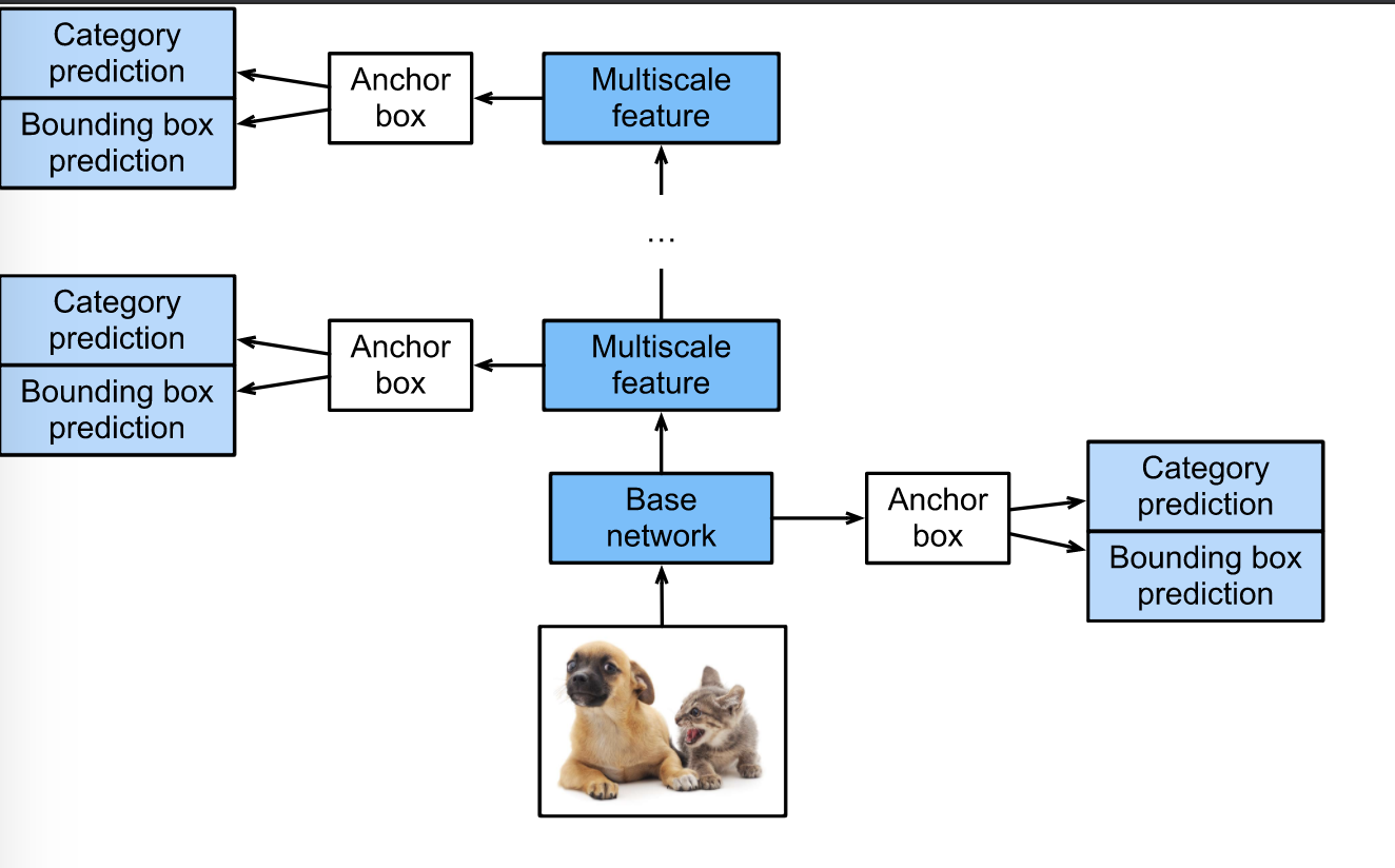
So overall, in a region prediction network, the input is an image, output is a (long) sequence of anchor boxes + categories.

We will only briefly dwell upon training the above architecture. The category prediction layer can be trained using cross entropy loss. The Jaccard similarity metric, unfortunately, cannot be directly used as a training loss since it is non-differentiable. Instead, the offset prediction layer can be trained using MSE (L2-loss) or MAE (L1-loss). In practice, a hybrid of these two losses called the Huber loss is used; this looks like $L2$ near zero (to maintain differentiability) and $L1$ away from zero.

Based on the above idea, many different types of RPN’s have been proposed, and the differences are in the details depending on flavor/efficiency:

• SSD (single-shot detection)
• R-CNNs
• Fast/Faster R-CNNs

One final comment: the above approach predicts rectangular bounding boxes. The alternative is to assign a category to each pixel, which gives higher precision to the localization output. This is called semantic segmentation.

There are both benefits and disadvantages of semantic segmentation versus regular bounding box detection. The pros are that pixel-level localization is potentially achievable via semantic segmentation. The cons are that large amounts of training data for semantic segmentation are considerably more difficult to acquire (one can intuitively see that labeling a bounding box is easy, but accurately labeling a semantic map can be challenging).