Lecture 6: Recurrent Neural Nets

In which we introduce deep networks for modeling time series data.

Recurrent Neural Networks

Thus far, we have mainly discussed deep learning in the context of image processing and computer vision. Let us now turn our attention to a different set of applications that involve text. For example, consider natural language processing (NLP), where the goal might be to:

• perform document retrieval: used in database- and web-search;

• convert speech (audio waveforms) to text: used in Siri, or Google Assistant;

• achieve language translation: used in Google Translate,

• map video to text: used in automatic captioning,

among a host of other applications.

Let us think about trying to use the tools we have developed so far to solve the above types of problems. Recall the kind of tools we have been using: thinking of data as real-valued vectors/arrays; representing entries of this array as nodes in a network; recursively applying arithmetic operations (organized in the form of layers); training the parameters of each layer; and so on.

Immediately we run into problems. For example, a document (or any other type of text object) is a string of characters, so how do we encode them into real-valued vectors? The naive approach would be to perform one-hot encoding of each character, just as how we encoded categorical labels in classification; but is this the best we can do? Should we instead try to model words, and if yes, then should we one-hot-encode words instead? Defining how to represent text is the first challenge.

Setting this question aside, a second challenge arises in the context of designing neural architectures for processing text data. If we think of representing the characters in a sentence into a linear vector/array, notice that the contents of the vector exhibits both short range as well as long-range dependencies. The short range dependencies encode relationships between characters in a word, or relationships between adjacent words; it is reasonable that one can capture this via a convnet.

But the long range dependencies are harder to model, and in a lot of languages the start of a sentence may have relevance to the end of a sentence. (Example: “The cow, in its full glory, jumped over the moon” – the subject and object are at two opposite ends of the sentence.) These kinds of non-local interactions are not easily captured by convnets, and therefore we need a new approach.

Markov and n-gram models

Before delving into neural nets for text processing, let us first discuss some classical methods. We will assume that text can be represented as a sequence of numerical symbols $w_1, w_2, \ldots$ where the symbols represent characters, words, or whatever model we define.

Classically, the tools to solve NLP problems were probabilistic language models. If we consider any sequence $w = (w_1,w_2,\ldots,w_d)$, then the goal would be to estimate the probability distribution:

\[P(w) = P(\{w_1, w_2, \ldots, w_T\})\]

From basic probability, we can factorize this distribution as:

\[P(w) = \Pi_{t=1}^T P(\{w_t | w_{t-1}, w_{t-2}, \ldots w_1\})\]

So the likelihood of any given sequence appearing depends on the conditional probability of a word given the appearance of the previous several words.

These probabilities, in principle, can be empirically estimated given a very large corpus of training data. However, in practice such estimates can be noisy (or even intractable, given the combinatorial explosion in the number of possible word combinations). To alleviate this, it is typical to make the (first-order) Markov model assumption, which states that the likelihood of each word only depends on the previous word in the sentence:

\[P(w) = P((w_1,w_2,\ldots,w_T)) = P(w_1) \cdot P(w_2 | w_1) \cdot \ldots P(w_T | w_{T-1}) .\]

Now the conditional probabilities are relatively easier to estimate: if we have $n$ words in the dictionary then we need to estimate roughly $O(n^2)$ probabilities. This is large but not intractable.

The first-order Markov assumption unfortunately ignores dependencies across time beyond a single hop. If we were being brave, we could extend it to two, or three, or $n$ previous words – these are called bigram, trigram, or n-gram models. But realize that as we introduce more and more dependencies across time, the probability computations quickly become large.

Recurrent architectures

An elegant way to resolve the time dependency issue and introduce long(er) range dependencies is via the notion of a latent variable called the state. We will rely on the following approximation:

\[P(\{w_t | w_{t-1}, w_{t-2}, \ldots w_1\}) \approx P(\{w_t | h_{t-1} \})\]

where $h_t$ is a hidden variable that approximately encodes all history up to the current instant. In general, we can assume that the state $h_t$ is a function of the previous state and the current input: $h_t = f(h_{t-1}, x_t)$.

Let us interpret this in the context of neural nets. Thus far, we have strictly used feedforward connections while discussing neural network architectures. Let us now introduce a new type of neural net with self-loops which acts on time series, called the recurrent neural net (RNN). In reality, the self-loops in the hidden neurons are computed with unit-delay, which really means that the state of the hidden unit at a given time step depends both on the input at that time step, and the state at the previous time step. The mathematical definition of the operations are as follows:

\[\begin{aligned} h^{t} &= \sigma(U x^{t} + W h^{t-1}) \\ y^{t} &= \text{softmax}(V h^{t}). \end{aligned}\]

So, historical information is stored in the output of the hidden neurons, across different time steps. We can visualize the flow of information across time by “unrolling” the network across time.

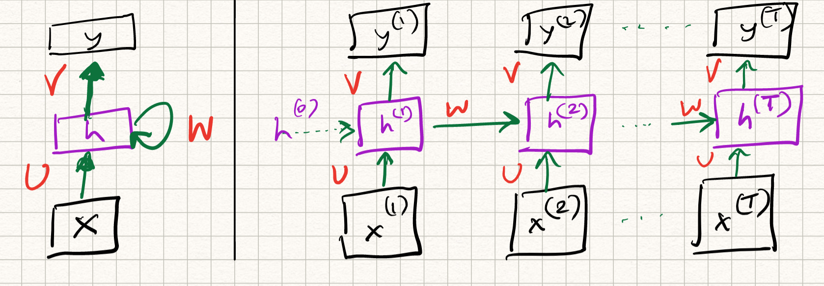
Observe that the layer weights $U, W, V$ are constant over different time steps; they do not vary. Therefore, the RNN can be viewed as a special case of deep neural nets with weight sharing.

Loss functions and metrics

Let us recall our three-step recipe for machine learning. Having defined a model (or a representation), we now have to define a goodness of fit. For text, there are a couple of options. The training loss is typically chosen as the cross-entropy (recall that we are trying to approximate the probability of an output symbol/token given previous inputs). So if $y^t$ is the predicted output and $g^t$ is the one-hot encoding of the ground truth, then we can write out:

\[l(y^t, g^t) = - \sum_i g_i^t \log y_i^t = - \log y_{I(g)}^t\]

where $I(g)$ is the index corresponding to the true word, and the overall loss is given by averaging over the entire training corpus:

\[L(\theta) = \frac{1}{T} \sum_{t=1}^T l(y^t, g^t) = - \frac{1}{T} \sum_t \log y_{I(g)}^t (\theta) .\]

In practice, this can be very hard to compute for large datasets, so this is broken down into batches (usually sentences). There are additional complications while computing gradients which we discuss below.

Evaluation of a given model is done via a quantity called perplexity, which happens to be related to the loss that we defined above. Perplexity is an information-theoretic concept that measures how well a probability model predicts a given object/symbol. It is defined as the exponent of the cross-entropy of the final model measured over the predictions made over a validation dataset:

\[\text{Perplexity} = \exp \left( - \frac{1}{T} \sum_t \log y_{I(g)}^t \right)\]

If there is a lot of certainty about what the model is predicting, then the probability distribution is peaked around the right output, the cross-entropy is 0, and the perplexity is 1. If the model is spitting out random words, the probability distribution is likely going to be uniform and the perplexity is going to be equal to the number of tokens in the vocabulary (exercise: why is this?). A good prediction model achieves lower perplexities.

Backpropagation through time

Again, training an RNN can be done using the same tools as we have discussed before: variants of gradient descent via backpropagation. The twist in this case is the feedback loop, which complicates matters. To simplify this, we simply unroll the feedback loop into $T$ time steps, and perform backpropagation through time for this unrolled (deep) network. We need to be careful when we apply the multivariate chain rules while computing the backward pass, but really it is all about careful book-keeping; conceptually the algorithm is the same.

Here is a more concrete description of the backprop updates. Let’s just ignore all matrix-vector multiplies (the calculus becomes complex) and just pretend that everything (input, output, hidden state) is a scalar. There are three sets of weights we need to figure out: the weights mapping input to the state ($u$), the weights mapping the state to itself ($w$), and the weights mapping the state to the output ($v$).

Remember that these weights are constant across time, so even if we unroll the network out to $T$ steps, there is a massive amount of weight-sharing going on. The chain rule gives us:

\[\begin{aligned} \frac{\partial L}{\partial w} &= \frac{1}{T} \sum_{t=1}^T \frac{\partial l^t}{\partial w} \\ &= \frac{1}{T} \sum_{t=1}^T \frac{\partial l^t}{\partial y^t} \frac{\partial y^t}{\partial h^t} \frac{\partial h^t}{\partial w} \end{aligned}\]

The first and second factors above are easy to calculate (it’s just the derivative of the cross-entropy and the soft-max). However, the last term is tricky. By definition,

\[h^t = \sigma(u x^{t} + w h^{t-1}) := f(w, h^{t-1})\]

Therefore, the derivative of $h^t$ with respect to $w$ has two components:

\[\frac{\partial h^t}{\partial w} = \frac{\partial f(w, h^{t-1})}{\partial w} + \frac{\partial f(w, h^{t-1})}{\partial h^{t-1}} \cdot \frac{\partial h^{t-1}}{\partial w} .\]

If we define a sequence $a_t := \frac{\partial h^t}{\partial w}$, then each $a_t$ depends on $a_{t-1}$, which in turn depends on $a_{t-2}$, and so on. This induces a recurrence relation for $a_t$. So to accurately compute gradients with respect to $w$, we need to perform backprop all the way to the start of time. In practice this is far too cumbersome and we usually just truncate after a certain number of time steps.

(Observe that this problem did not come up in regular feed-forward networks – the gradients at any layer only depended on the forward pass activations and the backward pass messages at that layer).

Even more troubling is the fact there is a multiplicative factor linking the terms $a_t$ and $a_{t-1}$. This has the effect of a geometric series: if the factor is greater than one on average across time, then the gradients explode, while if the factor is lesser than one on average across time, then the gradients vanish.

Stabilizing RNNS training and extensions

Vanishing/exploding gradients are a major headache in deep learning, and are even more pertinent in RNNs (which, by design, require unrolling over several time steps). One way to solve this problem is called gradient clipping where we simply ignore the magnitude of the gradient and normalize it to some norm $\alpha$ that is kept constant:

\[g \leftarrow \alpha \frac{g}{\|g\|} .\]

As you can imagine this is sub-optimal since it may lead to erroneous gradient updates. But at least the numerics are stable.

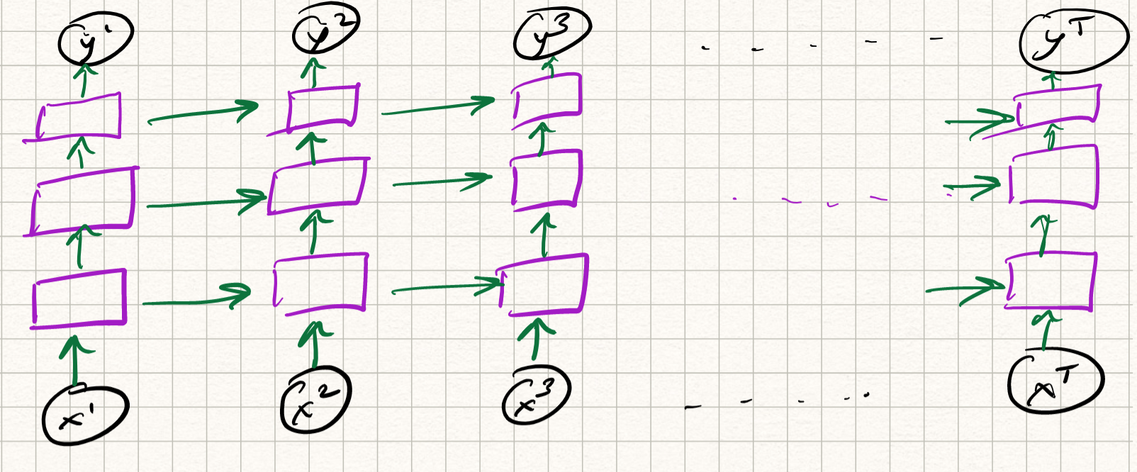
The alternative approach is to redesign the architecture itself. Notice the above example is for a single-layer RNN (which itself – let us be clear — is a deep network, if we imagine the RNN to be unrolled over time). We could make it more complex, and define a multi-layer RNN by computing the mapping from input to state to output itself via several layers. The equations are messy to write down so let’s just draw a picture:

Depending on how we define the structure of the intermediate layers, we get various flavors of RNNs:

• Gated Recurrent Units (GRU) networks
• Long Short-Term Memory (LSTM) networks
• Bidirectional RNNs

and many others. This gives us a lot of flexibility as to how to ensure that the gradient information propagates across several time steps.

LSTMs are the most well-known among the above architectures, but GRU’s are a bit simpler to explain formally so let’s do that (refer to the textbook for LSTMs if you are interested). The idea is similar: we interpret the state as the memory of a recurrent unit, and hence would like to also somehow decide whether certain units are worth memorizing (in which case the state is updated), and others are worth forgetting (in which case the state is reset). Let us define two gating operations, called “reset” ($r$) and “update” ($z$):

\[r^t = \sigma(U_r x^t + W_r h^{t-1}), z^t = \sigma(U_z x^t + W_z h^{t-1})\]

which both look like a regular state-update equation. Now, ordinarily in an RNN, as we discussed in the beginning of this lecture, we would update the state as:

\[h^{t} = \sigma(U x^{t} + W h^{t-1}) .\]

But in the GRU, we define the candidate state as:

\[\tilde{h}^{t} = \sigma\left(U x^{t} + W (h^{t-1} \odot r^t)\right)\]

with the intuition being that if the reset gate is close to 1, then this looks like a regular RNN unit (i.e., we retain memory), while if the reset gate is close to 0, then this looks like a regular perceptron/dense layer (i.e., we forget).

Now, the update gate tells us how much memory retention versus forgetting needs to happen:

\[h^t = h^{t-1} \odot z^t + \tilde{h}^{t} \odot (1 - z^t) .\]

Whenever the update gate is close to one, we retain the old state; whenever it is close to zero, the state is over-written.