Lecture 7: Transformers
In which we introduce the Transformer architecture and discuss its benefits.
Attention Mechanisms and the Transformer
Motivation
Attention models/Transformers are the most exciting models being studied in NLP research today, but they can be a bit challenging to grasp – the pedagogy is all over the place. This is both a bad thing (it can be confusing to hear different versions) and in some ways a good thing (the field is rapidly evolving, there is a lot of space to improve).
I will deviate a little bit from how it is explained in the textbook, and in other online resources: see Section 10 in the textbook for an alternative treatment.
Recall where we left off: general RNN models. They look like this:
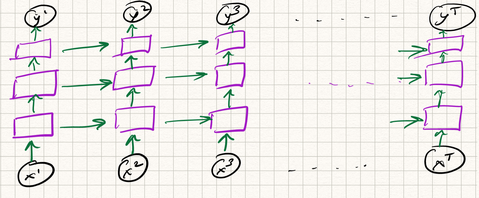 { width=90% }
We discussed some NLP applications that are suitable to be solved by RNNs. These include:
- next symbol/token prediction
- sequence classification
but there are several NLP applications for which RNN-type models are not the best. These include:
- neural machine translation (NMT)
- sentence generation
Consider, for example, the English sentence:
- “How do you like the weather today”?
and its German translation:
- “Wie finden sie das Wetter heute?”
While the two sentences are rather similar (both are Germanic languages) We find some subtle differences here. One is the difference in the number of words: the German version has one less word. The second is the order of the words – the pronoun “you” comes before the verb “like” in English but the pronoun “sie” after the verb “finden” in German. Both are examples of misalignment, and language translation has to frequently deal with small/local misalignments of this nature.
RNNs are not amenable to dealing with misalignments. The main reason is that RNNs (fundamentally) are sequence-to-symbol models: they output symbols one after the other based on the sequence seen so far. In NMT the outputs are not single tokens but sequences of tokens, each of which may depend on several parts of input sequence (both forwards and backwards in time) with long-range dependencies. How do we fix this problem? Let us consider a few different solution approaches.
Attempt 1. Model tokens as entire sentences, not words (i.e., build the language model at the sentence level, not at the word- or character-levels). This, of course, is not feasible – due to combinatorial explosion, the number of possible sentences becomes extremely large very quickly.
Attempt 2. A second approach is to use bidirectional RNNs. The idea is simple: read the input sequence both backwards and forwards in time. This way we will get two sets of hidden states. We can concatenate both states to decode the output. This is fine, but still does not capture very long range dependencies.
Attempt 3: Encoder-decoder architectures. Delay producing any output in the beginning. Just compute the states recursively until the last state (which is the “global” context/memory variable which captures the entire sequence). This is called the encoder. Then feed it to the input again to produce outputs. This is called the decoder. This is a fine idea but same issues with gradient vanishing, low ability of final state to capture overall context etc.
Attempt 4: Why only final state? Take all intermediate encoder states, store all of them as context vectors to be used by the decoder. This is getting better, but still too complex. There are encoder states, decoder states, decoder inputs \ldots getting way too complex. Also, it would be nice to figure out which parts of the input sequence influenced which other parts, so that we get a better understanding of the context. But how to assign “influence scores” systematically?
Self-Attention
This is the point where papers-blogs-tweets-slides etc start talking about keys/values and attention mechanisms and everything goes a bit haywire. Let’s just ignore all that for now, and instead talk about something called self-attention. The use of the “self-“ prefix will become clear later on.
Here is how it is defined. We have a set (not sequence, order does not matter right now) of input data points ${x_1, x_2, \ldots, x_n}$. They can all be $d$-dimensional vectors. We will produce a set of outputs ${y_1, y_2, \ldots, y_n}$, also $d$-dimensional vectors:
\[y_i = \sum_{j=1}^n W_{ij} x_j\]i.e., each output is a weighted average of all inputs where the weights $W_{ij}$ are row-normalized such that they sum to 1.
Crucially, the weights here are not the same as the (learned) parameters in a neural network layer. Instead, they are derived from the inputs. For example, one option is that we choose the weights to be dot-products:
\[w_{ij} = x_i^T x_j\]and apply the softmax function so that we get row-normalization:
\[W_{ij} = \frac{\exp{w_{ij}}}{\sum_j \exp{w_{ij}}}\]and use these weights to construct the outputs. That’s basically self-attention in a nutshell. In fact, this is all we will need to understand transformers/BERT/GPT etc.
Notice a few fundamental differences between regular convnets/RNNs and the operation we discussed above:
- Convnets map single inputs to single outputs. In self-attention, we map sets of inputs to sets of outputs, and by design, the interaction between data points is captured.
- RNNs map inputs seen thus far to single outputs. In self-attention, we are not limited to tokens/symbols only seen in the past.
- Until now, nothing is learnable here. This is an entirely deterministic operation with no free parameters. You can think of $x_i$ being features/embeddings that were learned “upstream” before being fed into the self-attention layer. We will add a few learnable parameters to the layer itself shortly.
- Observe that the operation is permutation-equivariant: if I permute the order of $x$, the output of $y$ is exactly the same, but permuted. This can pose challenges in NLP where permutations may result in completely different meanings. We will fix this shortly.
Before we proceed, why does this operation even make sense?
One interpretation is as follows: suppose we restrict our attention to linear models (so the output has to be a linear combination of the inputs). Say we were performing an NMT task that was translating “The cat sat on the hat” from English to German. One could represent each word in this sentence with an embedding/token.
However, there is a lot of redundancy in natural languages. Certain words (the, on) are common words that are not informative/correlated. Other words (cat, hat) are similar (both nouns). Words may be grouped according to subject-object relationships or subject-predicate relationships. It would be useful if the model automatically “grouped” similar words together. That would allow both better context and better training. The dot product provides a mechanism for automatically figuring out this kind of grouping.
OK, now let’s generalize the self-attention operation a little bit.
In the above definition of the self-attention layer, observe that each data point $x_i$ plays three roles:
- It is compared with all other data points to construct weights for its own output $y_i$ (i.e., in the dot-product example above, the sequence of weights $w_{i 1} = x_i^T x_1, w_{i 2} = x_i^T x_2, \ldots, w_{i n} = x_i^T x_n $).
- It is compared with every other data point $x_j$ to construct weights for their output $y_j$ (i.e., the weight $w_{1i} = x_1^T x_i, w_{2i} = x_2^T x_i$, \ldots).
- Once all the weights $w_ij$ have been constructed, it is used to finally synthesize each actual output $y_1, y_2, \ldots, y_n$.
These three roles are called the query, key, and value respectively. To make these roles distinct, let us add a few dummy variables:
\[\begin{aligned} q_i &= x_i, \\ k_i &= x_i, \\ v_i &= x_i \end{aligned}\]and then write out the output as:
\[w_{ij} = q_i^T k_j, \qquad W_{ij} = \text{softmax}(w_{ij}), \qquad y_i = \sum_j W_{ij} v_j .\]This is a lot of responsibility for each data point. Let’s make the life of each vector easier by adding learnable parameters (linear weights) for each these three roles. For numerical reasons, we also scale the dot-product (this does not change intuition at all).
Therefore, we get:
\[\begin{aligned} q_i &= W_q x_i, \qquad k_i = W_k x_i, \qquad v_i = W_v x_i \\ w_{ij} &= q_i^T k_j / \sqrt{d}, \qquad W_{ij} = \text{softmax}(w_{ij}), \qquad y_i = \sum_j W_{ij} v_j . \end{aligned}\]We can think of each of the $W_q$, $W_k$, $W_v$ as learnable projection matrices that defines the roles of each data point.
One last complication. We can concatenate different self-attention mechanisms to give it more flexibility. This is the same analogy as choosing multiple filters in a convnet layer. This is called multi-head self-attention. We can index each head with $r = 1, 2, \ldots$, so that we get learnable parameters $W^r_q$, $W^r_k$, $W^r_v$. We get independent outputs for each head and then combine everything using a linear layer to produce the outputs. So we finally get:
\[\begin{aligned} q^r_i &= W^r_q x_i, \qquad k^r_i = W^r_k x_i, \qquad v^r_i = W^r_v x_i \\ w^r_{ij} &= \langle q^r_i, k^r_j \rangle / \sqrt{d}, \qquad W^r_{ij} = \text{softmax}(w^r_{ij}), \qquad y^r_i = \sum_j W^r_{ij} v_j, \\ y_i &= W_y \text{concat}[y^1_i, y^2_i, \ldots]. \end{aligned}\]and there we have it. The entire (multi-head) self-attention layer. We will denote the above $x$-to-$y$ mapping as follows:
\[[y_1, y_2, \ldots, y_n] = \text{Att}([x_1, x_2, \ldots, x_n])\]Quick back-story on the nomenclature. These names query, key, value come from a key-value data structure. If we give a query key and match it to a database of available keys, then the data structure returns the corresponding matched value. The analogy is similar in attention mechanisms, except that the matching is done via dot-products (and the softmax ensures that it is a soft-matching, and every key in the database is matched to the query to some extent).
This also relates to the name “self-attention”. Recall our original discussion in the beginning of this lecture when we started discussed encoder/decoder architectures. We had recurrent neural networks taking the input ${x_i}$ and doing complicated things to get encoder context vectors ${h_i}$ and decoder states $s_i$. Then we were computing “influence scores” to figure out which words were relevant for (or “attend to”) which output. One mechanism proposed for doing this was to compute dynamic context scores:
\[c_i = \sum_{j} \alpha_{ij} h_j\]where $\alpha$ represented the alignment weights. This was called an attention mechanism, and early NMT papers used a shallow feedforward network (called an attention layer) to compute these alignment weights:
\[\alpha_{ij} = W_1 \text{tanh}(W_2 [h_i, s_j])\]followed by a softmax. Notice the similarities between what we discussed so far and the above formulation. A seminal paper in 2017 called “Attention is all you need” dramatically simplified things and showed that self-attention is enough – you could interpret contexts quite well in NLP tasks if we just let the input data tokens attend to themselves.
Transformers
We now use the self-attention layer described above to build a new architecture called the Transformer. The Transformer architecture now forms the backbone of the most powerful language models yet built, including BERT and GPT-2/3.
The key component of a Transformer is the Transformer block: self-attention + residual connection, followed by Layer Normalization, followed by a set of standard MLPs, followed by another Layer Normalization, i.e., something like this:
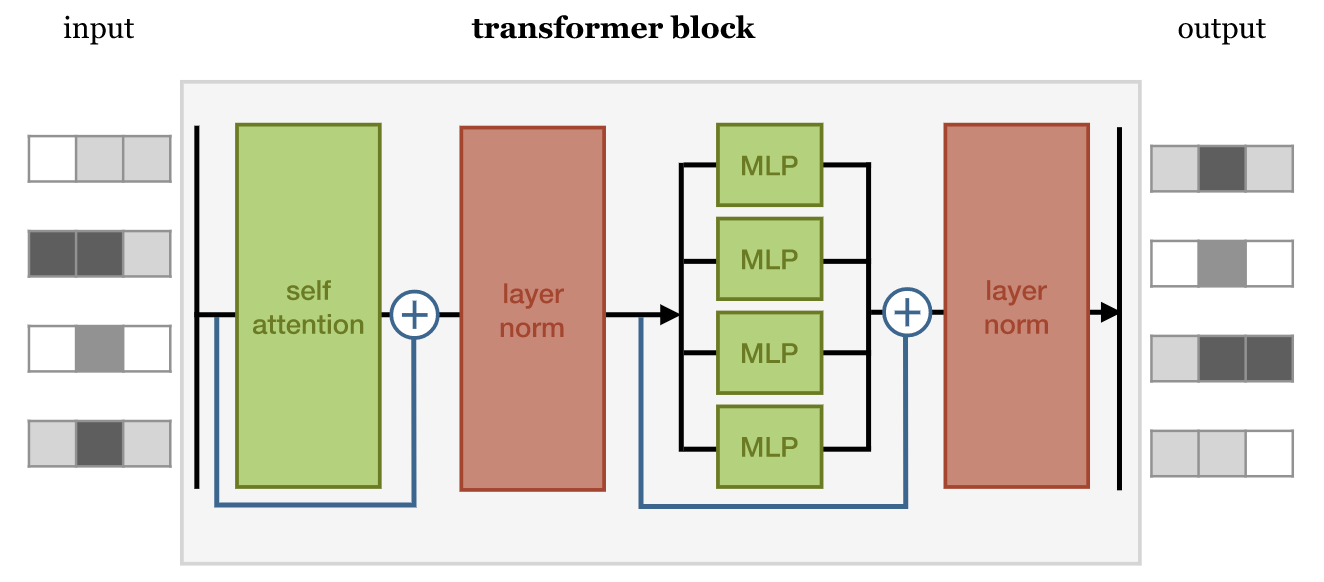
Observe that this architecture is completely feedforward, with no recurrent units. Therefore, gradients do not vanish/explode (by construction), and the depth of the network is no longer dictated by the length of the input (unlike RNNs). Multiple transformer blocks can then be put together to form the transformer architecture.
Transformers: Wrapup
One part that we didn’t emphasize too much in the previous lecture is the fact that unlike sequence models (such as RNNs or LSTMs), self-attention layers are permutation-equivariant. This means that sentences of the form:
“Jack gave water to Jill”
and
“Jill gave water to Jack”
will learn the exact same features. In order to incorporate positional information, some more effort is needed.
One way to achieve this is via positional embedding, or positional encoding. We create, in addition to the word embedding, a vector that encodes the location of the token. This vector can either be learned (just as word embeddings – see below) or just fixed. The latter is typically used in Transformer architectures.
What kind of positional encodings are useful? One-hot encoding the position is possible (although quickly becomes cumbersome – can you reason why this is the case?). Just adding an integer feature encoding the position is fine too, although we may run into scale/dynamic range issues, sinc the value of the feature can become very large for one sequences. A common approach is to use sinuisoidal encoding:
\[p_t = [sin(\omega_1 t); sin(\omega_2 t); \ldots sin(\omega_d) t]\]where $\omega_k = \frac{1}{10000^{k/d}}$ represents different frequencies. Thus the values of the positional encoding vector are always bounded, and because of the periodic nature of the definition this can be applied for any choice of $d$ and $t$.