Lecture 8: Applications in NLP

In which we see the power of deep networks in natural language processing.

In our discussion on deep learning for text, we have mainly focused on the middle part of this picture:

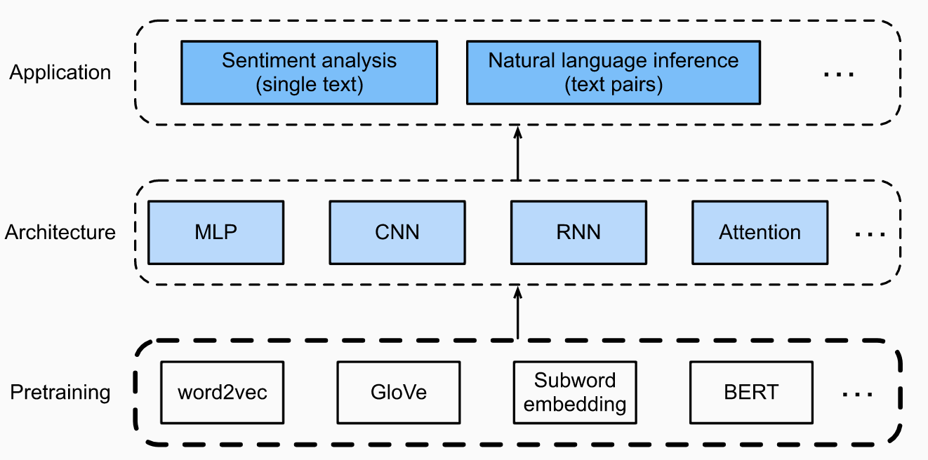
All neural network models assume real-valued vector inputs, and we have assumed that there is some magical way to convert discrete data (such as text) to a form that neural networks can process.

Today we will focus on the bottom part. Where do the word encodings come from? And how do they interact with the rest of the learning?

word2vec

The easiest way to encode words/tokens into real-valued vectors is one that we have already used for image-classification type applications: one-hot encoding.

Pros: this is dead simple to understand and implement.

Cons: there are two major drawbacks of using one-hot encodings.

• Each encoding can become very high dimensional. By definition, the encoded vectors are now the size of the vocabulary/dictionary. At the character level this is fine; at the word level it becomes very difficult; and at any higher level the space of symbols becomes combinatorially large.
• More than just computation: one-hot encodings do not capture semantic similarities (all words are equally far in L1/L2/Hamming distance than every other word). It would be nice to have similar words share similar features (where the meaning of “similar” depends on the language and/or context).

This was recognized by early NLP researchers. In the mid-2000s, a host of encoding methods were proposed, includng Latent semantic analysis (LSA), singular value decomposition (SVD). All of these were superseded by Word2vec, which came up in the early 2000s.

Word2vec is a word encoding framework that uses one of two approaches: skip-grams and continuous bag-of-words.

Skip-grams

In skip-grams, each word has two vector embeddings: $v_i$ and $u_i$. Let us first motivate why we need two such embeddings. As a running example, we will keep in mind a sentence such as:

“It is raining right now”.

and imagine it being represented as a sequence of words $x_1, x_2, x_3, x_4, x_5$.

We already discussed $n$-grams briefly before while motivating language models. For $n=2$, these are the joint probabilities

\[P(x_1,x_2), P(x_2,x_3), ...,\]

each of which can be empirically calculated by counting the number of co-occurrences of pairs of words in a database. Equivalently, it is easier to express this in terms of conditional probabilities

\[P(x_2 | x_1), P(x_3 | x_2), ...\]

The term “skip-gram” comes from the fact that we consider conditional probabilities that are not-consecutive, i.e., words can be skipped over. (The reason for exploring relationships between non-consecutive words goes back to the non-local, long-range dependency structure of natural languages.) In this case, the factorization is done with respect to the “center” (or “target”) word of the sequence; the other words are called “context” words. So the above factorization becomes:

\[P(x_1 | x_3) \cdot P(x_2 | x_3) \cdot P(x_4 | x_3) \cdot P(x_5 | x_3)\]

Intuitively, these probabilities tell us: “if a word $x_i$ appears in a sentence, how likely is it that the word $x_j$ will appear in its vicinity?” Here, “vicinity” would mean a window of some fixed size.

Having defined non-local conditional probabilities, the algorithmic question now becomes: how to estimate them? Again, one could just use the frequency of co-occurence counts in some large text corpus. However, we will depart from the standard approach, and instead train a simple neural network that predicts

\[P(x_j | x_i).\]

The network will be two layers deep (i.e., a single hidden layer of neurons with linear activations), followed by a softmax.

Some more details about this network. Say we have a dictionary of $N$ words. The input is a one-hot encoding $x_i$ of any given word $i$ (so, $N$ input neurons). The output is a vector of pre-softmax logits (so, $N$ output neurons). We can imagine (say) a hidden layer of $d$ (linear) neurons. So if we call $V \in \mathbb{R}^{d \times N}$ and $U \in \mathbb{R}^{d \times N}$ the two layers, then the conditional probability of any context word given the center is given by:

\[\begin{aligned} P(x_j | x_i) &= \text{softmax}(U^T V x_i) \\ &= \text{softmax}(U^T v_i ) \\ &= \text{softmax}([u_1^T v_i; u_2^T v_i; \ldots u_N^T v_i]) . \end{aligned}\]

So examining the rows of $U$ and $V$ give us precisely what we want – the word embeddings for the target and the context words respectively. Typically, $d \ll N$, so the embedding dimension is much smaller than the size of the vocabulary.

Using the rows of $U$ and $V$ as embeddings also intuitively makes sense: similar words/synonyms should give us similar output probabilities, and in order for two outputs to be similar, both target and context probabilities must match.

How do we train this network? First, we need to define a loss function. We can just use the standard cross-entropy loss, where the network is fed pairs of words (one-hot encoded) as data-label pairs. So for a particular pair of target-context words $i$ and $j$, we get the loss term:

\[l(i,j) = u_j^T v_i - \log\left(\sum_j \exp(u_j^T v_i)\right)\]

whose derivative can then be used to update all the weights.

There are a more few issues here to be considered. In English, for example, there are about $N = 10K$ commonly used words. So we already have approximately $6M$ weights to learn. Second, training can be extremely slow, since for every sample pair we have to touch all the weights. The word2vec paper did a few extra hacks (hierarchical softmax, negative sampling) to make this work, which we won’t dive into here – more details in an NLP course perhaps. See Chapter 14 of the textbook if you are interested.

Continuous Bag of Words (CBOW)

The CBOW model is very similar to the skip-gram model, so we won’t get into too much detail. THe main difference is that the CBOW model flips things around: instead of the center word defining the context, the context words are used to predict the target. So the conditional probabilities become:

\[P(x_3 | x_1, x_2, x_4, x_5)\]

which cannot be easily factorized the way we did so above. But the expression remains similar, if we approximate the embedding of the context as the (vector) average of the individual embeddings:

\[P(x_i | x_1, \ldots x_j \ldots) = \frac{\exp(u_i^T \text{Ave}(v_j))}{\sum_i \exp(u_i^T \text{Ave}(v_j))} .\]

Given this approximation of the conditional probabilities, the training is done just the same way as described above using the cross-entropy loss.

Which embedding is better? Both are roughly equivalent and we could use one or the other.

GloVe

The main problem with the word2vec framework is that both skip-gram and CBOW models rely on predicting output probabilities, and hence have to be trained with the cross-entropy loss.

For very large dictionaries, calculating cross-entropy can be troublesome: each gradient update requires computing softmaxes (and hence calculating all the outputs and marginalizing over them). Global vector (GloVe) embeddings resolve this in a slightly different manner. The idea is to use matrix factorization (a la PCA), and since it is not neural network-based we won’t go into too much detail here: take an NLP class if interested. The main steps are as follows:

• We construct a word-context co-occurrence matrix and try to factorize it using PCA (i.e., find the low-rank decomposition that minimizes the reconstruction loss).

• Not trivial, but this is a very sparse matrix! Can train using SGD type methods.

• Word distributions have a long tail, so very common words will dictate the loss function. To make things more equitable, log-probabilities are used.

• In practice, a modified weighted form of the reconstruction loss is used:

\[L(U,V,b,c) = \sum_{i,j} f(x_{ij}) (u_i^t v_j + b_i + c_j - \log x_{ij})^2\]

where $f(x_{ij}) = 1$ for reasonable $x_{ij}$ but quickly goes to 0 if $x_{ij}$ gets close to zero. This avoids the possibility that large (negative) values in the log-probabilities significantly influence the loss function.

ELMO, BERT, and GPT-2

While word2vec and GloVe represented step-changes in our ability to build sophisticated language models, they have now largely been surpassed by more modern techniques — ELMo, BERT, and GPT. Fortunately, we now have all the ingredients to understand them. The details are a bit hairy (a lot of engineering has gone into finetuning each of them) so we will only stick to high-level intuition and descriptions, while relegating the specifics to the textbook (Chapter 15).

ELMo

The main problem with GloVe/word2vec is that the word embeddings are context-independent. Recall that if we want to get a skip-gram embedding of a word, we one-hot encode it and look at the corresponding input- and output-layer weights in the above two-layer architecture.

However, words (particularly in languages such as English) are context-dependent. E.g. consider a sentence such as “Fish fish fish” — there are three identical words here, but the context shows that each has rather different meanings. Can we somehow get embeddings that not just look at word-level semantics but their usage in a given sentence?

ELMo (Embeddings from Language Models) does this. Just as how we motivated RNNs/LSTMs as possible architectures that can capture context in a sequence of inputs, similarly we can replace the simple feedforward architecture of word2vec with recurrent architectures.

Specifically, ELMo proposes to produce word embeddings by looking at the entire sentence both left-to-right and right-to-left. It achieves this via bi-directional LSTMs: it looks at the hidden layer representations (states) for both the left-to-right and right-to-left LSTMs and takes a weighted linear combination of them as the word embedding for each word in the input. The weights are left as trainable parameters used by downstream tasks (such as classification or sentence prediction) for further fine-tuning.

The choice of loss function is important; ELMo uses next-word-prediction (NWP) as the task of choice using the cross-entropy loss.

BERT

The next natural progression was to replace the bidirectional LSTM encoding used by ELMo with Transformers. This led to BERT (bidirectional encoder representations from transformers). The main ingredients (over and above those described above) include:

• Replacing LSTMs with transformer blocks. The output of each encoder layer in each token’s path can be viewed as a feature embedding of that toen.

• The loss function/training task used to learn the embeddings is for next-sentence prediction (NSP) which is shown to be transferable to many tasks.

• To encourage generalizability, a technique called masked self-attention is used: random words in a sentence are masked/zeroed out. This is similar to Dropout, which we have seen in the context of training feedforward nets.

• BERT also uses word piece tokenization, which is somewhere in between character-level and word-level encoding. This is useful for languages like English. For example, the world “Walking” is broken into two pieces: “walk” and “ing”, each of which are tokenized.

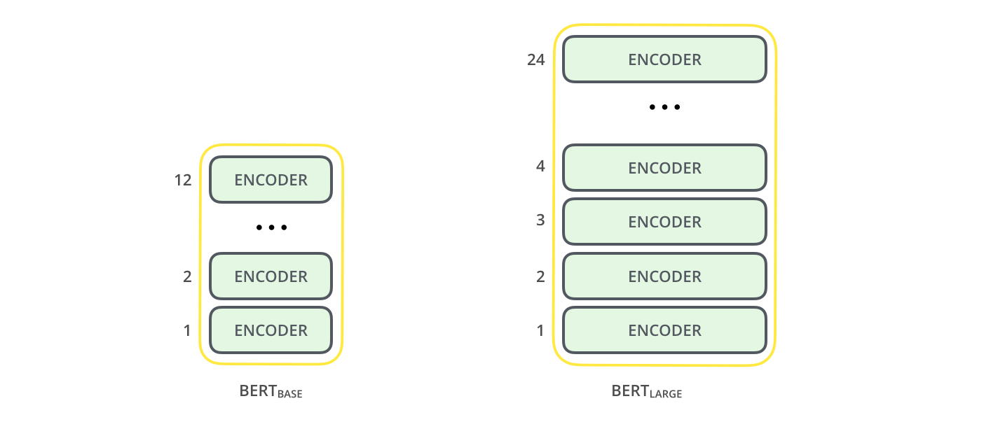
• There are two BERT models, which differ in the depth (number of encoder blocks) used in the Transformer architecture.

• BERT is now adopted by Google Search in most of their supported languages.

GPT-2

This line of work culminated in GPT-2 (GPT = Generative Pre-Training). Its successor (GPT-3) is possibly the most advanced language model currently present, but is closed-source.

A key difference with BERT is that GPT-2 uses masked auto-regressive self-attention, so tokens are not allowed to peek at words to the right of them.

GPT-2 also used much deeper architectures than BERT, and was trained on extremely massive datasets (called the OpenWebText Corpus).

Other hacks: similar to BERT, GPT uses word piece tokenization. GPT-2 used something called Byte Pair encodings that uses compression algorithms to figure out how to chop up regular words into tokens.

Summary

There you have it: a brief summary of modern neural architectures for NLP (and sequential data more broadly).

Among the many applications they support: apart from regular classification-type problems (such as sentiment analysis or named entity recognition), the above models support:

• Language synthesis – as used by chatbots and the like.
• Summarization: models such as GPT-2 can read a wikipedia article (without the intro paragraph) and be asked to summarize the intro.
• Similar architectures can be fine-tuned to perform music synthesis (such as synthetic midi file generation).