Lecture 2: Neural Nets

In which we discuss what neural networks are, how to train them, and how to use them once trained.

Neural Networks: Architecture, training, and prediction

In the previous lecture, we learned how shallow models (such as linear regression or perceptrons) can be viewed as special primitives called neurons, which form the building blocks of neural networks. The high level idea is to imagine each machine learning model in the form of a computational graph that takes in the data as input and produces the predicted labels as output. For completeness, let us reproduce the graphs for linear and logistic regression here.

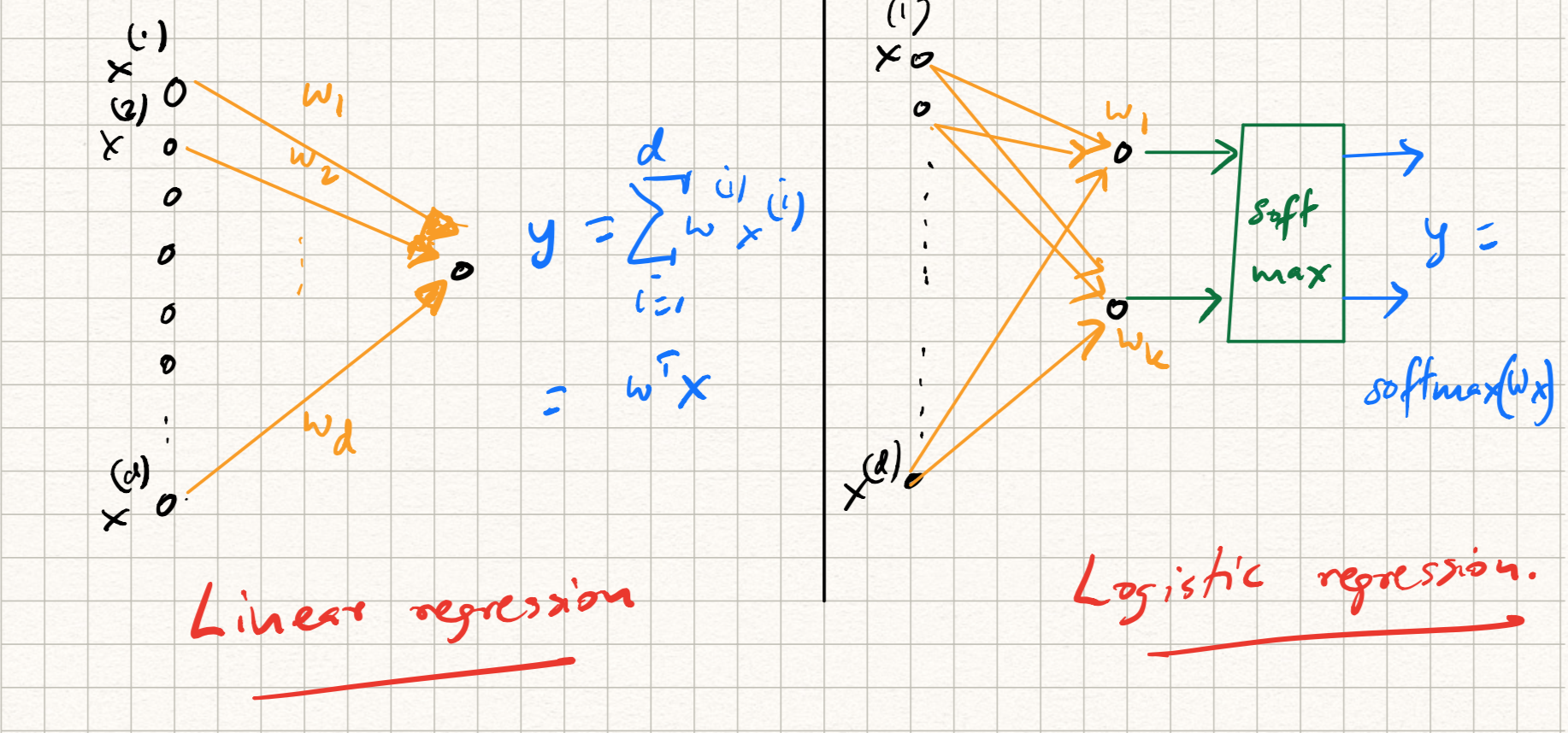
If we do that, we will notice that the graph in the above (linear) models has a natural feed-forward structure; these are instances of directed acyclic graphs, or DAGs. The nodes in such a DAG represent inputs and outputs; the edges represents the weights multiplying each input; outputs are calculated by summing up inputs in a weighted manner. The feed-forward structure represents the flow of information during test time; later, we will discuss instances of neural networks (such as recurrent neural networks) where there are feedback loops as well, but let us keep things simple here.

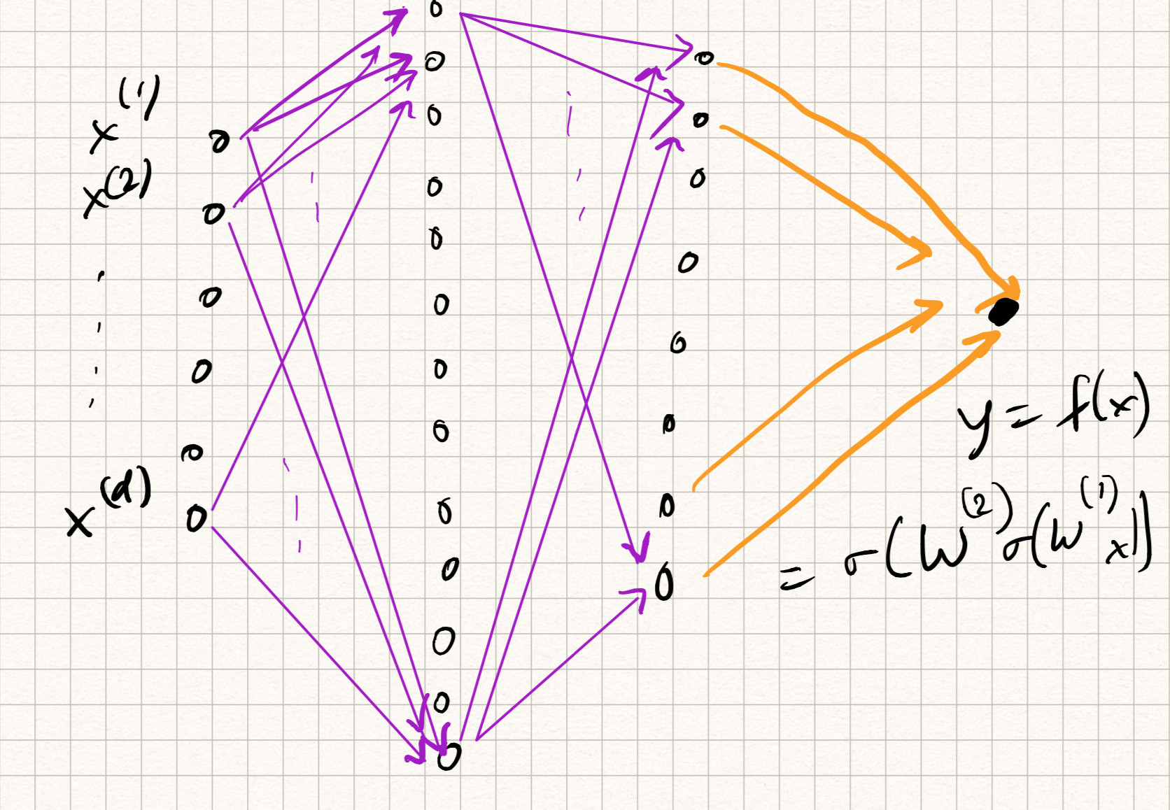
Let us retain the feed-forward structure, but now extend to a composition of lots of such units. The primitive operation for each “unit”, which we will call a neuron, will be written in the following functional form:

\[z = \sigma(\sum_{j} w_j x_j + b)\]

where $x_j$ are the inputs to the neuron, $w_j$ are the weights, $b$ is a scalar called the bias, and $\sigma$ is a nonlinear scalar transformation called the activation function. So linear regression is the special case where $\sigma(z) = z$, logistic regression is the special case where $\sigma(z) = 1/(1 + e^{-z})$, and the perceptron is the special case where $\sigma(z) = \text{sign}(z)$.

A neural network is a feedforward composition of several neurons, typically arranged in the form of layers. So if we imagine several neurons participating at the $l^{th}$ layer, we can stack up their weights (row-wise) in the form of a weight matrix $W^{(l)}$. The output of neurons forming each layer forms the corresponding input to all of the neurons in the next layer. So a 3-layer neural network would have the functional form:

\[\begin{aligned} z_1 &= \sigma^{1}(W^{1} x + b^{1}), \\ z_2 &= \sigma^{2}(W^{2} z_1 + b^{2}), \\ y &= \sigma^{3}(W^{3} z_2 + b^{3}) . \end{aligned}\]

Analogously, one can extend this definition to $L$ layers for any $L \geq 1$. The nomenclature is a bit funny sometimes. The above example is either called a “3-layer network” or “2-hidden-layer network”; the output $y$ is considered as its own layer and not considered as “hidden”.

Neural nets have a long history, dating back to the 1950s, and we will not have time to go over all of it. We also will not have time to go into biological connections (indeed, the name arises from collections of neurons found in the brain, although the analogy is somewhat imperfect since we don’t have a full understanding of how the brain processes information.)

The computational reason why neural nets are rather powerful is that they are “universal approximators”: a feed-forward network with a single hidden layer of finitely many neurons with suitably chosen weights can be used to approximate any continuous function. This works for a large range of activation functions. This property is called the Universal Approximation Theorem (UAT) and an early version can be attributed to Cybenko (1989). So for most prediction problems, if our goal is to learn an unknown prediction function $f$ for which $y = f(x)$, we can pretend that it can be approximated by a neural network, and learn its weights.

However, note that the UAT merely confirms the existence of a neural network as the solution for most learning problems. It does not address the practical issue of how to actually find a good network. Examining the theorem carefully indicates that even though we use just one hidden layer, we may need an exponentially large number of neurons even in moderate cases. So therefore, the UAT works for shallow, wide networks. To resolve this, the trend over the last decade has been to trade off between width and depth: namely, keep width manageable (typically, of similar size as the input) but concatenate multiple layers. (Hence the name “deep neural networks”, or “deep learning”).

Broadly, algorithmic questions in deep learning are of three flavors:

• How do we choose the widths, types, and number, of layers in a neural network?
• How do we learn the weights of the network?
• Even if the weights were somehow learned using a (large) training dataset, does the prediction function work for new examples?

The first question is a question of designing the representation (Step 1 in our general ML recipe) for a particular application. The second is a question of choice of loss function and training algorithm (Steps 2 and 3). The third is an issue of generalization. Intense research has occurred (and is still ongoing) in all three questions.

Neural network architectures

In typical neural networks, each hidden layer is composed of identical units (i.e., all neurons have the same functional form and activation functions).

Activation functions of neurons are essential for modeling nonlinear trends in the data. (This is easy to see: if there were no activation functions, then the only kind of functions that neural nets could model were linear functions). Typical activation functions include:

• the sigmoid $\sigma(z) = 1/(1 + e^{-z})$.
• the hyperbolic tan $\sigma(z) = (1 - e^{-2z})/(1 + e^{-2z})$.
• the ReLU (rectified linear unit) $\sigma(z) = \max(0,z)$.
• the hard threshold $\sigma(z) = \text{step}(z)$.
• the sign function $\sigma(z) = \text{sign}(z)$.

among many others. The ReLU is most commonly used nowadays since it does not suffer from the vanishing gradients problem (notice that all the other activation functions flatten out for large values of $z$, which makes it difficult to calculate gradients.)

There are also various types for layers:

• Dense layers – these are basically layers of neurons whose weights are unconstrained
• Convolutional layers – these are layers of neurons whose weights correspond to filters that perform a (1D or 2D) convolution with respect to the input.
• Pooling layers – These act as “downsampling” operations that reduce the size of the output. There are many sub-options here as to how to do so.
• Batch normalization layers – these operations rescale the output after each layer by adjusting the means and variances for each training mini-batch.
• Recurrent layers – these involve feedback connections.
• Residual layers – there involve “skip connections” where the outputs of Layer $l$ connect directly to Layer $l+2$.
• Attention layers – these are used in NLP applications,

among many others.

As you can see, there are tons of ways to mix and match various architectural ingredients to come up with new networks. How do we decide which recipe to use for specific applications and datasets is an open question. Good practice indicates the following thumb rule: just use architectures that have known to work for other similar domain applications. The majority of this course (once we are done with the basics) will be spent in exploring different architectures for different applications.

Gradient descent

Let us assume that a network architecture (i.e., the functional form of the prediction function $f$) has been decided upon. How do we learn its parameters (i.e., the weights and biases)?

To answer this question, we have to turn to Steps 2 and 3 of our recipe. First, we define a good loss function (where “goodness” is measured for the application at hand) and then find the weights/biases that minimize it. To actually find the minimum of any function, a canonical approach in applied math is to start at a given estimate, and iteratively descend towards new points with lower functional value. In mathematical terms, if we are at some estimate (say $\hat{w}$), suppose we found a direction $\Delta$ such that:

\[f(\hat{w} + \Delta) < f(\hat{w}) .\]

If we had an oracle that repeatedly gave us a new direction $\Delta$ for any $\hat{w}$ then we could simply update:

\[\hat{w} \leftarrow \hat{w} + \Delta\]

and iterate!

Fortunately, calculus tells us that for certain types of functions (i.e., smooth functions), the gradient at any point is a suitable descent direction; in fact, it points us in the direction of steepest descent. This motivates the following natural (and greedy) strategy: start at some estimate $w_k$, and iteratively adjust that estimate by moving in the direction opposite to the gradient of the loss function at $w_k$, i.e.,

\[w_{k+1} = w_k - \alpha_k \nabla L(w_k) .\]

The parameter $\alpha_k$ is called the step size, and controls how far we descend along the gradient. (The step size can be either constant, or vary across different iterations). In machine learning, $\alpha_k$ is called the learning rate.

At any point, if we encounter $\nabla F(w) = 0$ there will be no further progress. Such a $w$ is called a stationary point. If $F$ is smooth and convex, then all stationary points are global minima, and gradient descent eventually gives us the correct answer.

Before using this approach on neural nets, let us quickly use this idea for a shallow model (linear regression). It is not too hard to see that the mean-squared error loss is both smooth and convex (it is shaped like a parabola). Therefore, gradient descent is a reasonable approach for minimizing this type of function. If $L(w) = 0.5 |y - Xw |^2$, the iterates of gradient descent give:

\[\begin{aligned} w_{k+1} &= w_k + \alpha_k X^T (y - X w_k) \\ &= w_k + \alpha_k \sum_{i=1}^n (y_k - \langle w_k,x_i \rangle) x_i. \end{aligned}\]

Iterate this enough number of times and we are done. There is a nice interpretation of the above procedure: the update to the weights of the network is proportional to the cumulative prediction error made by all the samples.

Observe that the per-iteration computational cost is $O(nd)$, which can be several orders of magnitude lower than $O(nd^2)$ for large datasets. However, to precisely analyze running time, we also need to get an estimate on the total number of iterations that yields a good solution.

There is also the issue of step-size: what is the “right” value of $\alpha_k$? And how do we choose it? This is a major problem in ML and in the next lecture, we will talk about tuning the learning rate (and other tricks to make things work).

Stochastic gradient descent (SGD)

One issue with gradient descent is the uncomfortable fact that one needs to repeatedly compute the gradient. Let us see why this can be challenging. The gradient descent iteration for the least squares loss is given by:

\[w_{k+1} = w_k + \alpha_k \sum_{i=1}^n (y_i - \langle w_k, x_i \rangle) x_i\]

So, per iteration:

• One needs to compute the $d$-dimensional dot products
• by sweeping through each one of the $n$ data points in the training data set.

So even for linear regression, the running time is $\Omega(nd)$ at the very least. This is OK for datasets that can fit into memory. However, for extremely large datasets, not all the data is in memory, and even computing the gradient once can be a challenge. Imagine now doing this for very deep networks.

A very popular alternative to gradient descent is stochastic gradient descent (SGD for short). The idea in SGD is simple: instead of computing the full gradient involving all the data points, we approximate it using a random subset, $S$, of data points as follows:

\[w_{k+1} = w_k + \alpha_k' \sum_{i \in S} (y_i - \langle w_k, x_i \rangle) x_i .\]

The core idea is that the full gradient can be viewed as a weighted average of the training data points (where the $i^{th}$ weight is given by $y_i - \langle w_k, x_i \rangle$), and therefore one can approximate this average by only considering the average of a random subset of the data points.

The interesting part of SGD is that one can take this idea to the extreme, and use a single random data point to approximate the whole gradient! This is obviously a very coarse, erroneous approximation of the gradient, but provided we sweep through the data enough number of times the errors will cancel themselves out and eventually we will arrive at the right answer. (This claim can be made mathematically precise but we won’t go there.)

Here is the full SGD algorithm.

Input: Training samples $S = {(x_1, y_1), (x_2, y_2), \ldots, (x_n, y_n)}$.

Output: A vector $w$ such that $y_i \approx \langle w,x_i \rangle$ for all $(x_i, y_i) \in S$.

1. Initialize $w_0 = 0$.

2. Repeat:

   a. Choose $i \in [1,n]$ uniformly at random, and select $(x_i,y_i)$.

   b. Update:

   \[w_{k+1} \leftarrow w_k + \alpha_k (y_i - \langle w_k, x_i \rangle) x_i\]

   and increment $k$.

   While epoch $\leq 1,..,maxepochs$.

We won’t analyze SGD in great detail but will note that the step-size cannot be constant across all iterations (the reason for this is somewhat subtle). A good choice of decaying step size is the hyperbolic function:

\[\alpha_k = C/k .\]

One can see that the per-iteration cost of SGD is only $O(d)$ (assuming that the random selection can be done in unit-time, which is typically true in the case of random access memory). The price you typically pay is a greater number of iterations (compared to regular GD).

SGD is very popular, and lots of variants have been proposed. The so-called “mini-batch” SGD trades off between the coarseness/speed of the gradient update in SGD versus the accuracy/slowness of the gradient update in full GD by taking small batches of training samples and computing the gradient on these samples.

(S)GD and neural networks

The basic approach is similar to what we have seen before: we first choose a suitable loss function, and then use (the above variations of) gradient descent to optimize it. (For example, in a regression or classification setting, we might choose the cross-entropy loss.) Stack up all the weights and biases of the network into a variable $W$ Then, we first define:

\[L(W) = \sum_{i=1}^n l(y_i, f(x_i)) + \lambda R(W)\]

where $l(\cdot, \cdot)$ is the loss applied for a particular prediction and $R(\cdot)$ is an optional regularizer. Then, we train using GD (or more commonly, minibatch SGD):

\[W^{t+1} = W^{t} - \alpha^{t} \left( \sum_{i \in S} \nabla l(y_i, f_W(x_i)) + \lambda \nabla R(W) \right).\]

where $S$ is a minibatch of samples. So really, everything boils down to computing the gradient of the loss. As we will see below, this may become cumbersome.

Let us work out the gradient of the ridge regression loss (which is basically the mean-square error with an additional regularization term) for a single neuron with a sigmoid activation with a single scalar data point. The model is as follows:

\[\begin{aligned} z &= wx + b,~f(z) = \sigma(z),\\ L(w,b) &= 0.5 (y - \sigma(wx + b))^2 + \lambda w^2. \end{aligned}\]

Calculation of the gradient is basically an invocation of the chain rule from calculus:

\[\begin{aligned} \frac{\partial L}{\partial w} &= (\sigma(wx + b) - y) \sigma'(wx + b) x + 2 \lambda w, \\ \frac{\partial L}{\partial b} &= (\sigma(wx + b) - y) \sigma'(wx + b). \end{aligned}\]

Immediately, we notice some inefficiencies. First, the expressions are already very complicated (can you imagine how long the expressions will become for arbitrary neural nets?). Sitting and deriving gradients is tedious and may lead to errors.

Second, notice that the above gradient computations are redundant. We have computed $\sigma(wx + b)$ and $\sigma’(wx + b)$ twice, one each in the calculations of $\frac{\partial L}{\partial w}$ and $\frac{\partial L}{\partial b}$. Digging even deeper, the expression $wx + b$ appears four times. Is there a way to avoid repeatedly calculating the same expression?

The backpropagation algorithm

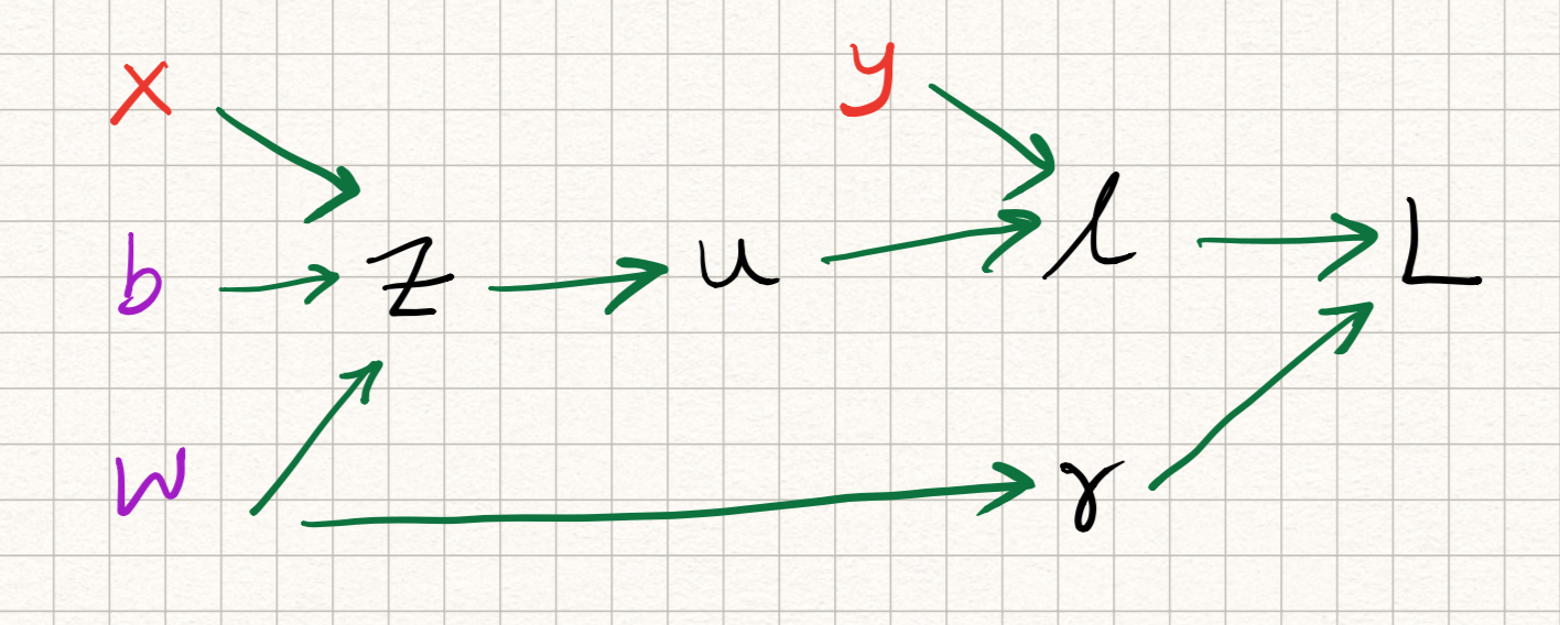
The intuition underlying the backpropagation algorithm (or backprop for short) is that we can solve both of the above issues by leveraging the structure of the network itself. Let us decompose the model a bit more clearly as follows:

\[\begin{aligned} z &= wx + b, \\ u &= \sigma(z), \\ l &= 0.5 (y-u)^2, \\ r &= w^2, \\ L &= l + \lambda r. \end{aligned}\]

This sequence of operations can be written in the form of the following computation graph:

{ width=90% }

Observe that the computation of the loss $L$ can be implemented via a forward pass through this graph. The algorithm is as follows. If a computation graph $G$ has $N$ nodes, let $v_1, \ldots, v_N$ be the outputs of this graph (so that $L = v_N$).

function FORWARD():

1. for $i = 1, 2, \ldots, N$:

   a. Compute $v_i$ as a function of $\text{Parents}(v_i)$.

Now, observe (via the multivariate chain rule) that the gradients of the loss function with respect to the output at any node only depends on what variables the node influences (i.e., its children). Therefore, the gradient computation can be implemented via a backward pass through this graph.

function BACKWARD():

1. For $i = N-1, \ldots 1$:

   a. Compute

   \[\frac{\partial L}{\partial v_i} = \sum_{j \in \text{Children}(v_i)} \frac{\partial L}{\partial v_j} \frac{\partial v_j}{\partial v_i}\]

Maybe best to explain via example. Let us revisit the above single neuron case, but use the BACKWARD() algorithm to compute gradients of $L$ at each of the 7 variable nodes ($x$ and $y$ are inputs, not variables) in reverse order. Also, to abbreviate notation, let us denote $\partial_x f := \frac{\partial f}{\partial x}$.

We get:

\[\begin{aligned} \partial_L L &= 1, \\ \partial_r L &= \lambda, \\ \partial_l L &= 1, \\ \partial_u L &= \partial_l L \cdot \partial_u l = u-y, \\ {\partial_z L} &= {\partial_u L} \cdot {\partial_z u} = \partial_u L \cdot \sigma'(z), \\ {\partial_w L} &= {\partial_z L} \cdot {\partial_w z} + {\partial_r L} \cdot {\partial_w r} = \partial_u L \cdot x + \partial_r L \cdot 2 w, \\ {\partial_b L} &= {\partial_z L} \cdot {\partial_b z} = {\partial_z L}. \end{aligned}\]

Note that we got the same answers as before, but now there are several advantages:

• no more redundant computations: every partial derivative depends cleanly on partial derivatives on child nodes (so, operations that have already been computed before) and hence there is no need to repeat them.

• the computation is very structured, and everything can be calculated by traversing once through the graph.

• the procedure is modular, which means that changing (for example) the loss, or the architecture, does not change the algorithm! The expressions for $L$ changes but the procedure for computation remains the same.

In all likelihood, you will not have to implement backpropagation by hand in real applications: most neural net software packages (like PyTorch) include an automatic differentiation routine which implement the above operations efficiently. But under the hood, this is what is going on.