Lecture 1: Introduction

In which we provide a brief crash course on machine learning.

Overview

Why machine learning, and why now?

As of today, ML (and more broadly, “AI” or “data science”) is an off-the-charts hot topic. Virtually every scientific, engineering, and social discipline is undergoing a major foundational shift towards an increasing use of AI. A major driver of this progress has been the development of DL tools and techniques, particularly over the last 5 years.

There are several reasons why this is the case; the foremost being that computing devices and sensors have pervasively been ingrained our daily personal and professional lives, and that it is easier and cheaper to acquire and process data than ever before. As we will learn later in the course, a common set of algorithmic tools in DL uses these devices to extract useful, actionable information from datasets of unprecedented sizes and varieties.

It is common to hear and read pithy newspaper headlines about AI, such as this:

“AI is the new electricity.”

or even

“AI is the new oil.”

It is true that a renewed focus on AI and data-driven analysis and decision making has had considerable impact on a lot of fields. It is equally true that several important questions remain unanswered, and that much of the deep learning tools used by practitioners are deployed as “black-boxes” with little-to-no understanding of what goes on under the hood.

The only way to place deep learning on a solid footing is to build it bottom-up from the first principles upwards; in other words, ask the same foundational questions that computer scientists would ask: correctness, soundness, efficiency, and so on. This course may not provide all the answers to these questions (much of which are still unknown!) but let’s treat this as a first step.

What is machine learning?

There is no unique answer. My own personal definition is the following diagram:

• Data –> (Machine learning system) –> Actionable information

To come up with a good ML system, there are three main computational ingredients.

• a representation of the system (also called an “ML model”)

• a measure of goodness (also called a “loss function” in machine learning).

• a method to optimize for this measure (also called a “training algorithm”).

Once we come up with such a (Machine learning system), we can use it to make predictions (also called “inference”).

All of the above assumes that the data itself obeys a certain mathematical form. A common approach in ML is to use vector spaces. Let us formalize this.

Vector spaces

In several applications, “data” usually refers to a list of numerical attributes associated with an object of interest.

For example: consider meteorological data collected by a network of weather sensors. Suppose each sensor measures:

• wind speed ($w$) in miles per hour
• temperature ($t$) in degrees Fahrenheit

Consider a set of such readings ordered as tuples $(w,t)$; for example: (4,27), (10,32), (11,47), $\ldots$

It will be convenient to model each tuple as a point in a two-dimensional vector space. More generally, if data has $d$ attributes (that we will call features), then each data point can be viewed as an element in a $d$-dimensional vector space, say $\mathbb{R}^d$.

Here are some examples of vector space models for data:

1. Sensor readings (such as the weather sensor example as above).

2. Image data. Every image can be modeled as a vector of pixel intensity values. For example, a $1024 \times 768$ RGB image can be viewed as a vector of $d = 1024 \times 768 \times 3$ dimensions.

3. Time-series data. For example, if we measure the price of a stock over $d = 1000$ days, then the aggregate data can be modeled as a point in 1000-dimensional space.

Properties of vector spaces

Recall the two fundamental properties of vector spaces:

• Linearity: two vectors $x = (x_1, \ldots, x_d)$ and $y = (y_1, \ldots, y_d)$ can be added to obtain: \(x + y = (x_1 + y_1, \ldots, x_d + y_d).\)

• Scaling: a vector $x = (x_1, \ldots, x_d)$ can be scaled by a real number $\alpha \in \mathbb{R}$ to obtain: \(\alpha x = (\alpha x_1, \ldots, \alpha x_d).\)

Vector space representations of data are surprisingly general and powerful. Moreover, several tools from linear algebra/Cartesian geometry will be very useful to us. Here are a few.

Norms. Each vector can be associated with a norm, loosely interpreted as the “length” of a vector. For example, the $\ell_2$, or Euclidean, norm of $x = (x_1, \ldots, x_d)$ is given by:

\[\|x\|_2 = \sqrt{\sum_{i=1}^d x_i^2}.\]

Similarly, the $\ell_1$, or Manhattan, norm of $x$ is given by:

\[\|x\|_1 = \sum_{i=1}^d |x|_i.\]

Distances. Vector spaces can be endowed with a notion of distance as follows: the “distance” between $x$ and $y$ can be interpreted as the norm of the vector $x-y$. For example, the $\ell_2$, or Euclidean, distance between $x$ and $y$ is given by:

\[\|x-y\|_2 = \sqrt{\sum_{i=1}^d (x_i - y_i)^2}.\]

One can similarly define the $\ell_1$-distance. The choice of distance will be crucial in several applications when we wish to compare how close two vectors are.

Similarities. These are, in some sense, the opposite of distances. Define the Euclidean inner product between vectors $x$ and $y$ as:

\[\langle x, y \rangle = \sum_{i=1}^d x_i y_i.\]

Then, the cosine similarity is given by:

\[\text{sim}(x,y) = \frac{\langle x, y \rangle}{\|x\|_2 \|y\|_2}.\]

The inverse cosine of this quantity is the generalized notion of angle between $x$ and $y$.

Warmup: Linear Models

Suppose we have observed data-label pairs ${(x_1,y_1),(x_2,y_2),\ldots,(x_n,y_n)}$ and there is some (unknown) functional relationship between $x_i$ and $y_i$. We will assume the label $y_i$ can be any real number. The problem of regression is to discover a function $f$ such that $y_i \approx f(x_i)$. (Later, we will study a special case known as binary classification, where the labels are assumed to be $\pm 1$). The hope is that once such a function $f$ is discovered, then for a new, so-far-unseen data point $x$, we can simply apply $f$ to $x$ to predict its label.

Examples include:

• predicting stock prices ($y$) from econometric data such as quarterly revenue ($x$)
• predicting auto mileage ($y$) from vehicle features such as weight ($x$). We have introduced this as a class lab exercise.
• forecasting Uber passenger demand ($y$) from population density ($x$) for a given city block
• … and many others.

As our simplest case, we assume a linear model on the function (i.e., the label $y_i$ is a linear function of the data $x_i$).

---

An aside: why should do we care about linearity? For starters, linear models are simple to understand and interpret and intuitively explain to someone else. (“If I double some quantity, my prediction doubles too..”) Linear models are also (relatively) easy from a computation standpoint. We will analytically derive below examples of linear models for a given training dataset in closed form.

From a mathematical perspective, if we recall the concept of Taylor series expansions, functions that arise in natural applications can often be locally expressed as linear functions. We will see later how Taylor series approximations arise all over the place in deep learning.

---

Let us focus on the case of high-dimensional (vector-valued) data. In this case, the functional form for the prediction made by linear models is as follows:

\[y_i = \langle w, x_i \rangle,~i=1,\ldots,n.\]

where $w \in \mathbb{R}^d$ is a vector containing all the regression coefficients.

(For simplicity, we have dropped the intercept term in the linear model. In ML jargon, this is called the bias, and can be handled analogously but the closed-form expressions below are somewhat more tedious.)

The second step is the loss function. Let us define the MSE loss in this case:

\[L(w) = \frac{1}{2} \sum_{i=1}^d (y_i - \langle x, w \rangle)^2,\]

For conciseness, we write this as:

\[L(w) = \frac{1}{2} \|y - Xw\|^2\]

where the norm above denotes the Euclidean norm, $y = (y_1,\ldots,y_n)^T$ is an $n \times 1$ vector containing the $y$’s and $X = (x_1^T; \ldots; x_n^T)$ is an $n \times d$ matrix containing the $x$’s, sometimes called the “data matrix”. Statisticians like to call this the design matrix.

In high dimensions, the vector of partial derivatives (or the gradient) of $L(W)$ is given by:

\[\nabla L(w) = - X^T (y - Xw) .\]

The above function $L(w)$ is a quadratic function of $w$. The value of $w$ that minimizes this (say, $w^*$) can be obtained by setting the gradient of $L(w)$ to zero and solving for $w$:

\[\begin{aligned} \nabla L(w) &= 0, \\ - X^T (y - Xw) &= 0, \\ X^T X w &= X^T y, \qquad \text{or}\\ w &= (X^T X)^{-1} X^T y . \end{aligned}\]

The above represents a set of $d$ linear equations in $d$ variables, and are called the normal equations. If $X^T X$ is invertible (i.e., it is full-rank) then the solution to this set of equations is given by:

\[w^* = \left(X^T X \right)^{-1} X^T y.\]

So there we have it – the solution to linear regression in closed form. Unfortunately, there are two issues here:

• Existence: If $n \geq d$ then one can generally (but not always) expect $X^T X$ to be invertible; if $n < d$, this is not the case and the matrix is singular, so the above expression is not valid.

• Computation: Computing $X^T X$ takes $O(dn^2)$ time, and inverting it takes $O(d^3)$ time. So, in the worst case (assuming $n > d$), we have a running time of $O(dn^2)$, which can be problematic for large $n$ and $d$. Can we do something simpler?

In the next lecture, we will develop an algorithm called gradient descent that will resolve both of these issues.

Classification and the perceptron

The perceptron algorithm was an early attempt to solve the problem of artificial intelligence. Indeed, after its initiation in the early 1950s, people believed that perfect AI was not far off. (Of course, that didn’t quite work out yet.) Let us see how our 3-step recipe described above applies here.

Step 1: Representation: The goal of the perceptron is to learn a linear model that can perfectly distinguish between two classes. In particular, the perceptron will output a vector $w \in \mathbb{R^d}$ and a scalar $b \in \mathbb{R}$ such that for each input data vector $x$, its predicted label is:

\[y = \text{sign}(\langle w, x \rangle + b).\]

If we assume that the learned separator $w$ is homogeneous and passes through the origin then $b = 0$. Geometrically, the boundary of the decision regions between the two classes is the hyperplane defined by:

\[\langle w, x\rangle = 0\]

and $w$ denotes a vector that is perpendicular to this hyperplane.

Step 2: Loss function: The next step is to define a measure of goodness. In classification applications, since the output is discrete/categorical, the mean-squared error is generally not meaningful. Instead, one can use, for example, the Hamming distance, which aggregates the number of

\[L(w) = \frac{1}{n} \sum_{i=1}^n \mathbf{1}(y_i \neq \text{sign}(\langle w, x \rangle + b)\]

where $\mathbf{1}$ denotes the indicator function that is 1 when the condition with the parenthesis is satisfied, and 0 otherwise.

Step 3: Optimization: We have been doing good so far, but now we come to a roadblock: staring at this a bit, we realize that there is no closed form expression for the minimizer of the above loss function!

Attempts to set the gradient to zero and solve for $w$ are not fruitful: observe that both the Hamming distance as well as the sign function are not differentiable, and hence the gradients may not even exist.

We could look to brute-force our way through it by examining all choices of $w$ and picking the best one, but we quickly run into computational intractability concerns here. We need a different class of algorithmic techniques (and indeed, computational concerns might have been the reason that the buzz around AI died down in the 60s).

We will see next lecture that a variant of the aforementioned gradient descent algorithm (called stochastic gradient descent) can resolve both these issues can elegantly solve the perceptron training problem.

From linear models to neural networks

With the above two examples in mind, let us try to make this connection between linear models and neural networks a bit more formal. The key concept linking these different models is to imagine the computations as being composed of layers in a directed graph.

For example, while training/testing a linear regression model, the following steps are involved:

• The input $x$ is dotted with a weight vector $w$, i.e., $\langle w, x \rangle$.
• The predicted output $\langle w, x \rangle$ is compared with the label $y$ using the squared error loss

\[l(y,w^T x) = 0.5 \|y - w^T x\|^2_2.\]

• Training is done by figuring out the best possible choice of $w$ that minimizes this loss.

Try building a graphical picture for the perceptron.

On the other hand, while training a ($k$-class) logistic regression model, we have an extra step:

• The input $x$ is dotted with $k$ weight vectors $w_j$.

• The (intermediate) output $z = (\langle w_1, x \rangle, \ldots, \langle w_k, x \rangle)$ is passed through a softmax layer to get the prediction:

  \[\hat{y} = \text{softmax}(z),~~\text{where}~~\hat{y}_j = \frac{\exp{\langle w_j, x \rangle}}{\sum\limits_{j=1}^k \exp{\langle w_j, x \rangle}}.\]
• The predicted output is compared with the label using cross-entropy loss:

\[l(y,\hat{y}) = - \sum_{i=1}^k y \log(\hat{y}).\]

Here, $y$ is a label indicator, or one-hot vector indicating the correct class.

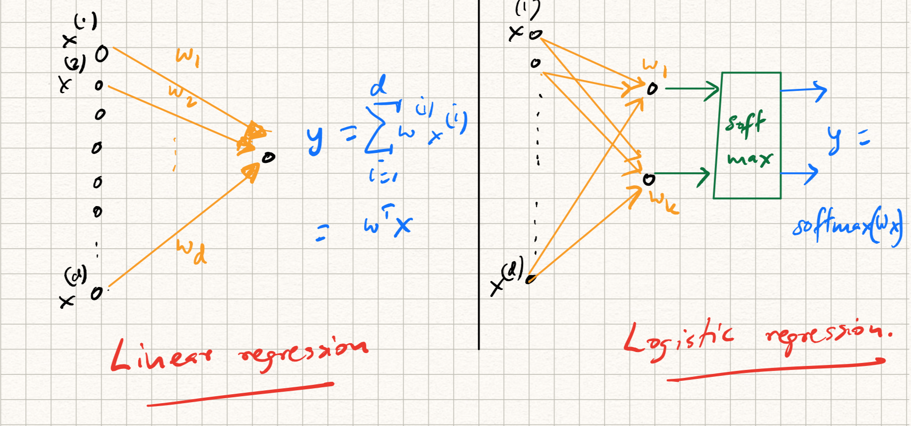
Each of the above procedures can be illustrated as a graph as illustrated in Figure 1. A shared picture starts to emerge:

• several standard ML models can be viewed as graphs;
• which are directed, acyclic, feedforward;
• the edges of the graph are associated with parameters (or weights) of the ML model,
• which can be iteratively, greedily updated via gradient descent.

As we will see in the coming two lectures, the core of modern deep learning systems consists of the very same steps discussed above.